Mode seeking in mean field VB for RSS + sparse prior

Using polynomial approximations to perform Bayesian regression

The RSS likelihood relates observed marginal effects to the unobserved effects of a joint model

\[\begin{align} \hat \beta \sim \mathcal N(SRS^{-1} \beta, SRS) \\ \beta \sim g(\cdot) \end{align}\]

Where we consider the problem of putting an i.i.d. prior on the entries of \(\beta\) and using a mean field approximation for variational inference.

Specifically, we put a spike and slab prior on \(\beta_j = b_j\gamma_j\) for \(j \in [p]\). Where \(b_j \sim N(0, \sigma^2)\) gives the distribution of non-zero effects, and and \(\gamma_j \sim Bernoulli(\pi)\). That is, the effect is non-zero with probability \(\pi\).

The problem we demonstrate, is that due to the mode matching behavior of the “reverse” KL divergence, which is minimized in variational inference, the posterior on \(q(\gamma_1, \dots, \gamma_p)\) will tend to concentrate instead of accurately representing uncertainty. Furthermore, due to strong dependence among the posterior means.

We work with a simplified version of RSS assuming we observe \(z\)-scores \(\hat z\).

\[ \begin{aligned} \hat z &\sim \mathcal N(Rz, R) \\ z_i &\sim \pi_0 \delta_0 + \pi_1 \mathcal N(0, \sigma^2) \end{aligned} \]

\[ q(z, \gamma) = \prod_j q(z_j, \gamma_j) \]

\[ \begin{aligned} ELBO(q_j) &= \mathbb E_{q_{-j}} \squarb{\log p(\hat z| z, R) + \log p(z_j) - \log q(b_l, \gamma_l)} + H(q_l) \\ &= \hat z_j (b_j \gamma_j) - \frac{1}{2} \left[ (b_j \gamma_j)^2 + 2 (b_j \gamma_j) \sum_{i \neq j} R_{ij} \mathbb E_{q_{-j}} \squarb{z_j} \right] + \log p(b_l | \gamma_l) + \log p(\gamma_l) + H(q_l) + C \end{aligned} \]

Then \(q(b_l | \gamma_l = 1) = N(\frac{\nu_j}{\tau_j}, \tau^{-1}_j)\) Where \(\nu_j = \hat z_j - \sum_{i\neq j} R_{ij} \alpha_i \mu_i\), and \(\tau_j = 1 + \sigma^{-2}_0\).

It’s easy to see that the best choice for \(q(b_l | \gamma_l = 0)\) is the prior, since all fo the data terms disappear, also noted here [(1)]

And \(q(\gamma_j) = Bernoulli(\alpha_j)\), where \(\log \left(\frac{\alpha_j}{1 - \alpha_j}\right) = \hat z \mu_j - \frac{1}{2} \left[\mu^2_j + \sigma^2_j + 2 \mu_j \sum_{i\neq j} R_{ij} \mu_i \alpha_i \right] + \log\left(\frac{\pi}{1 - \pi}\right)\).

Simulation

Code

#' @param q q(mu, var, alpha)
#' @param R LD matrix-- assumes diag(R) = rep(1, p)
#' @param tau0 prior effect variance
#' @param prior_logit p-vector with prior log odds for gamma = 1
rssvb <- function(zhat, q, R, tau0, prior_logit){
  # unpack
  mu <- q$mu
  var <- q$var
  alpha <- q$alpha

  p <- length(zhat)
  psi <- (R %*% (mu * alpha))[,1] # prediction
  for(i in 1:p){
    # remove effect of this variable
    psi <- psi - R[i,] * (mu[i]*alpha[i])

    # compute q(beta | gamma = 1)
    nu <- zhat[i] - psi[i]
    tau <- 1 + tau0
    mu[i] <- nu/tau
    var[i] <- 1/tau

    # logit <- zhat[i] * mu[i]
    #   - 0.5 * (psi[i] * mu[i] +  mu[i]^2 + var[i])
    #   -0.5 * tau0 * (mu[i]^2 + var[i]) + prior_logit[i]
    logit <- 0.5 * (mu[i]^2/var[i] + log(var[i]) + log(tau0)) + prior_logit[i]
    alpha[i] <- 1/(1 + exp(-logit))

    alpha[i]
    psi <- psi + R[i,] * (mu[i]*alpha[i])
  }
  return(list(mu=mu, var=var, alpha=alpha))
}

Code

sim_zscores <- function(n, p){
  X <- logisticsusie:::sim_X(n=n, p = p, length_scale = 5)
  R <- cor(X)
  z <- rep(0, p)
  z[10] <- 5
  zhat <- (R %*% z)[,1] + mvtnorm::rmvnorm(1, sigma=R)[1,]
  return(list(zhat = zhat, z=z, R=R))
}

init_q <- function(p){
  q = list(
    mu = rep(0, p),
    var = rep(1, p),
    alpha = rep(1/p, p)
  )
  return(q)
}

run_sim <- function(n = 100, p = 50, tau0=1, prior_logit = -3){
  sim <- sim_zscores(n = n, p = p)
  q <- init_q(p)
  prior_logit <- rep(prior_logit, p)
  for(i in 1:100){
    q <- with(sim, rssvb(zhat, q, R, tau0, prior_logit))
  }
  
  sim$q <- q
  return(sim)
}

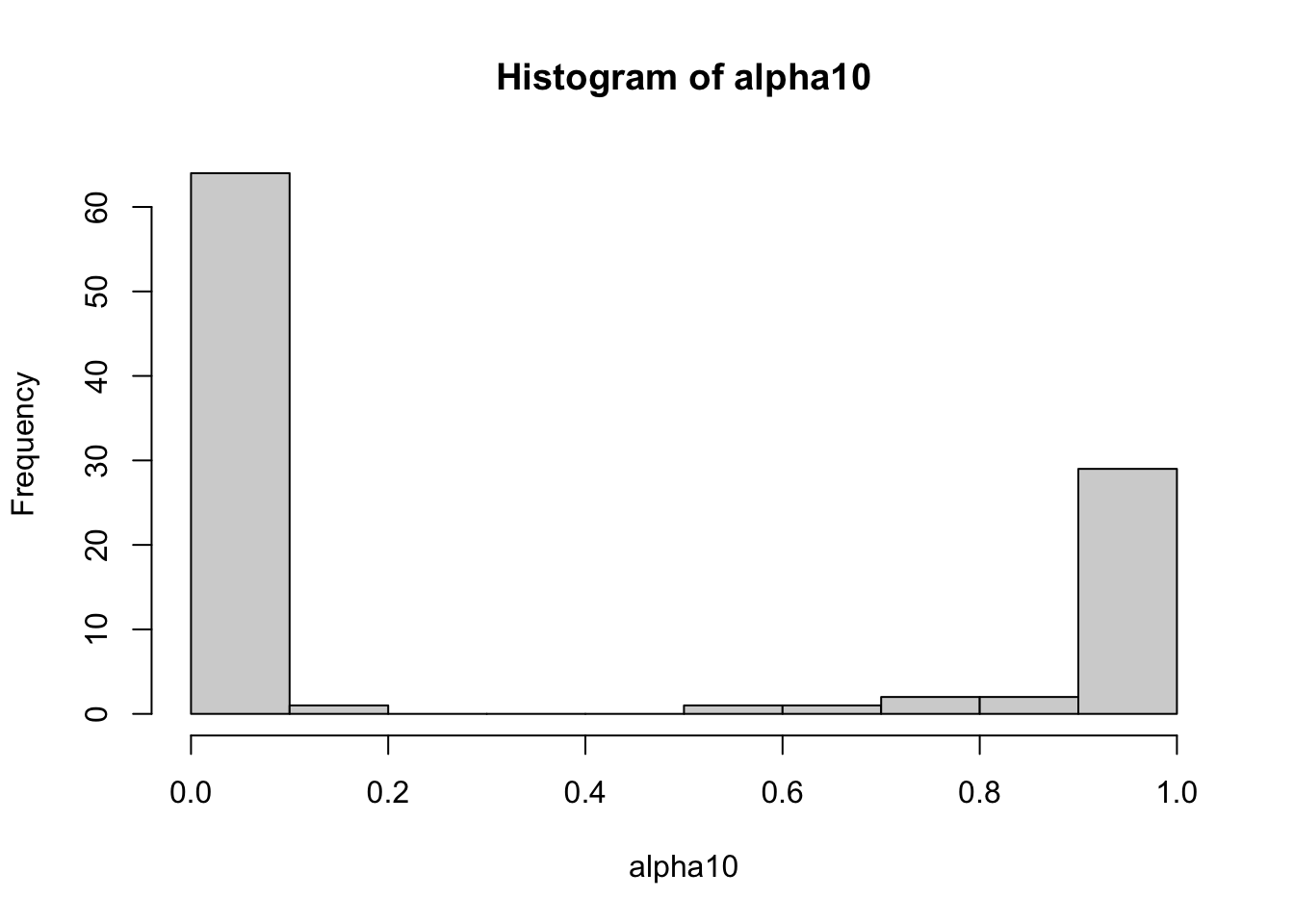
For 100 independent simulations, we simulate \(50\) dependent \(z\)-scores. The true non-zero \(z\)-score is at index \(10\) with \(\mathbb E[\hat z_{10}] = 5\). However, over half the time, the VB approximation confidently selects another nearby feature.

Code

set.seed(10)
sims <- purrr::map(1:100, ~run_sim(tau0=0.01))
max_idx <- purrr::map_int(1:100, ~which.max(sims[[.x]]$q$alpha))

alpha10 <- purrr::map_dbl(1:100, ~sims[[.x]]$q$alpha[10])
hist(alpha10)

Code

table(max_idx)

max_idx
 8  9 10 11 12 
 4 47 36 11  2 

Many small effects vs a few large effects

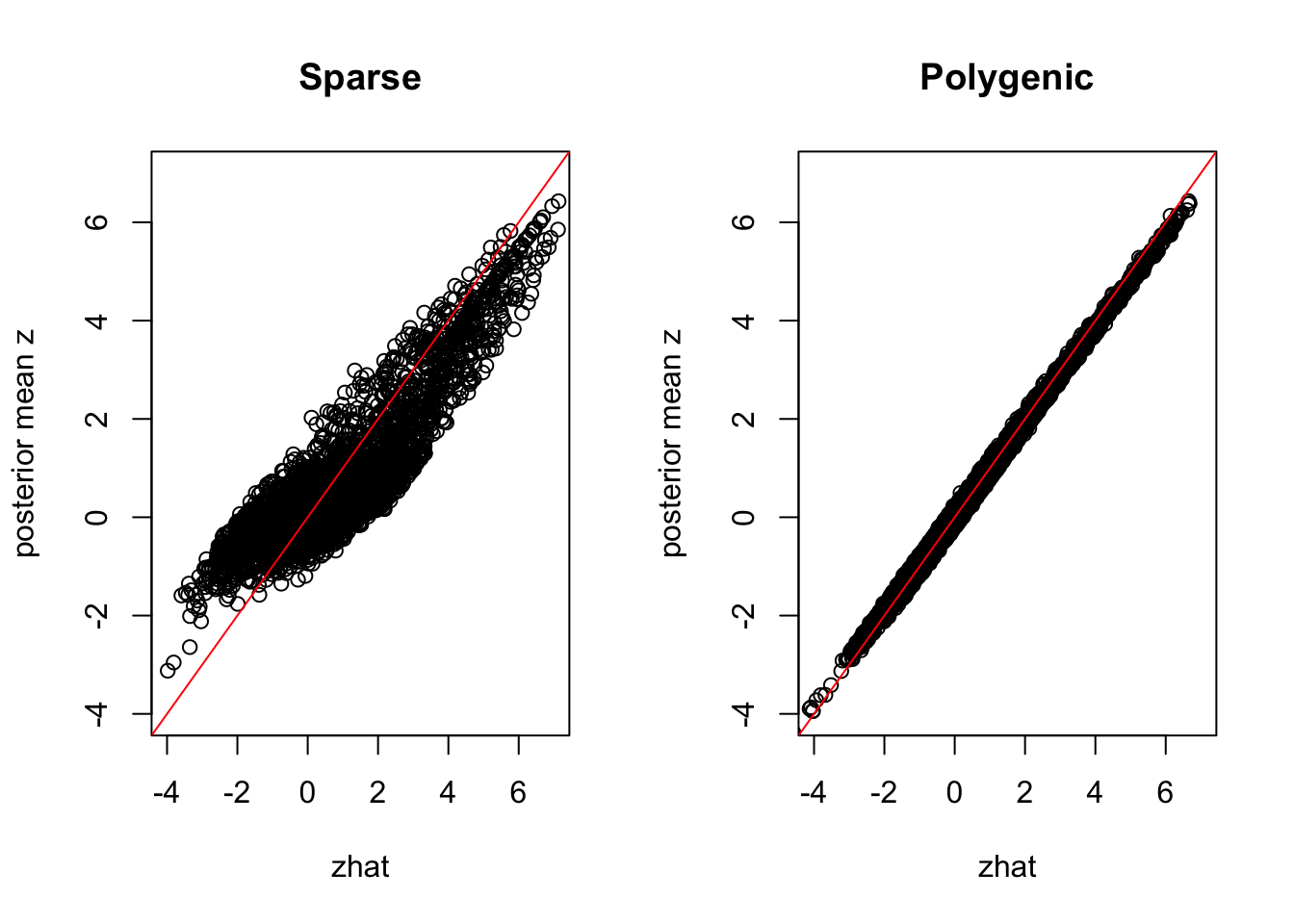
The interpretation of \(\sigma_0^2\) depends a lot on how polygenic the trait is. Even though we only simulate one non-zero effect, if we use a prior \(\pi_1 >> 0\) the model approaches a mean field approximation of ridge regression. Since ridge can estimate many small effects we get less shrinkage than if we enforce sparse architecture with \(\pi_1 \approx 0\).

Code

posterior_mean <- function(sim){
  return((sim$R %*% (sim$q$mu * sim$q$alpha))[, 1])
}

shrinkage_plot <- function(sims, ...){
  lims <- range(purrr::map(1:length(sims), ~sims[[.x]]$zhat))
  plot(
    sims[[1]]$zhat,
    posterior_mean(sims[[1]]),
    xlim = c(-4, 7),
    ylim = c(-4, 7),
    xlab = 'zhat',
    ylab = 'posterior mean z',
    ...
  )
  for(i in 1:100){
    points(sims[[i]]$zhat, posterior_mean(sims[[i]]))
  }
  abline(0, 1, col='red')
}

set.seed(10)

sim_sparse <- purrr::map(1:100, ~run_sim(tau0=0.1, prior_logit = -3))
sim_poly <- purrr::map(1:100, ~run_sim(tau0=0.1, prior_logit = 3))

par(mfrow=c(1,2))
shrinkage_plot(sim_sparse, main='Sparse')
shrinkage_plot(sim_poly, main='Polygenic')

References

1.

Titsias MK, Lázaro-Gredilla M. Doubly Stochastic Variational Bayes for non-Conjugate Inference.