More BF comparisons

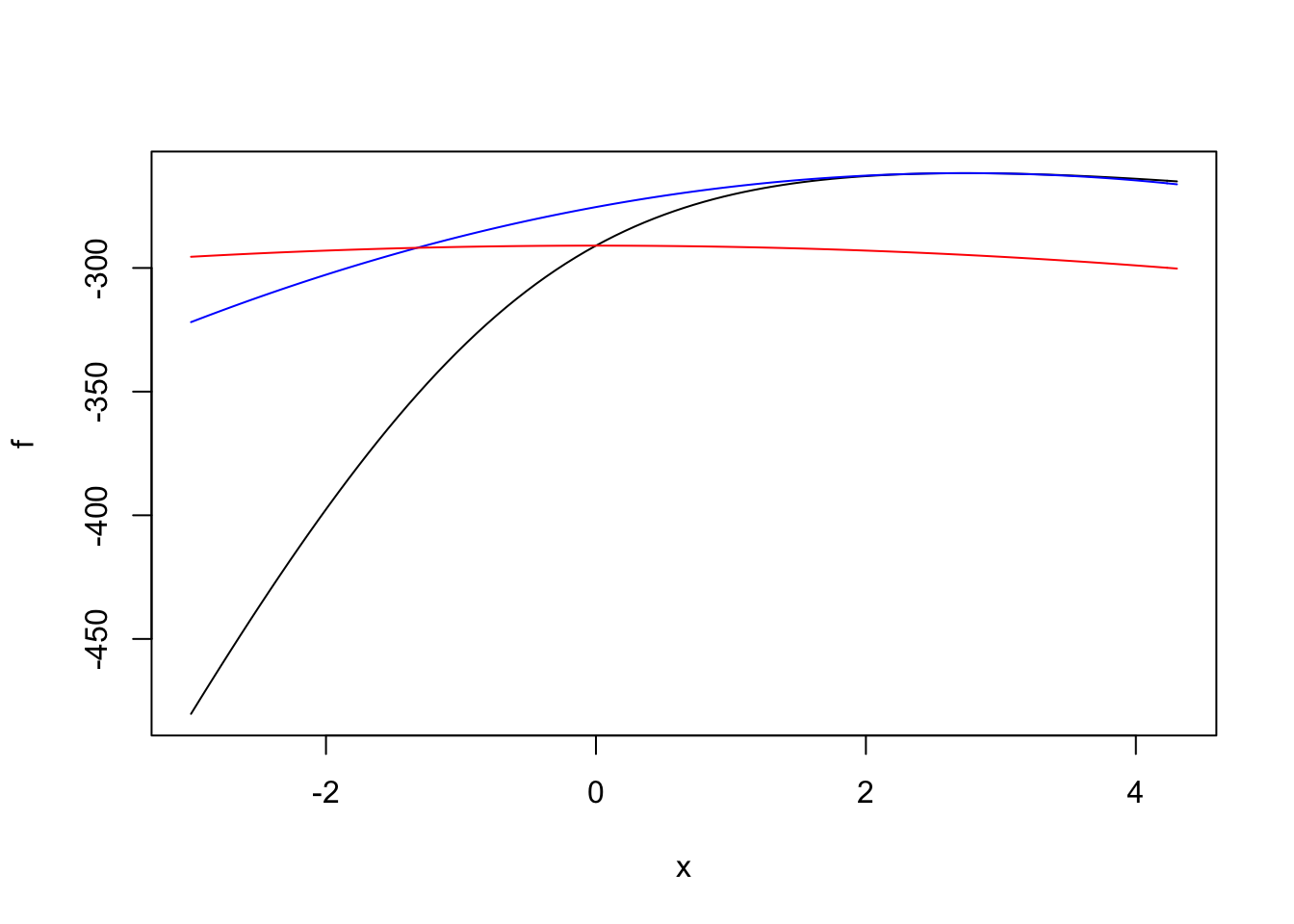
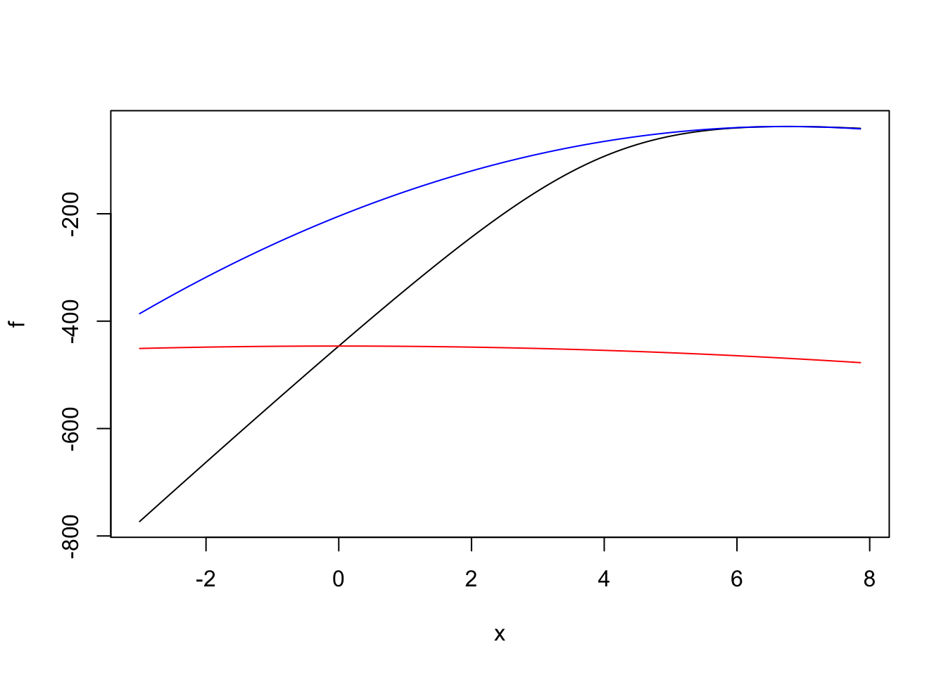
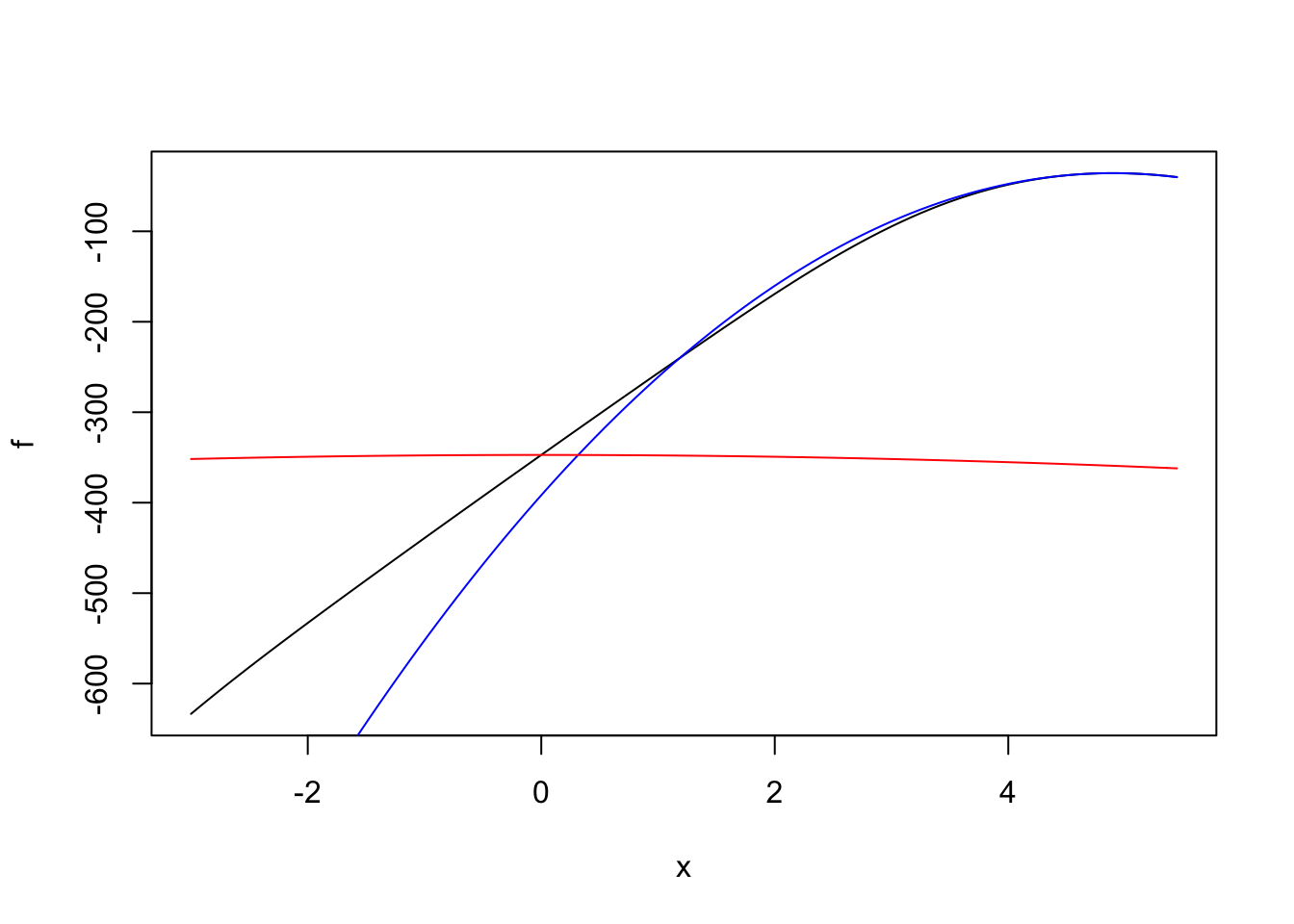
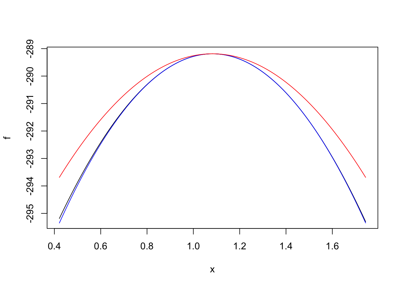
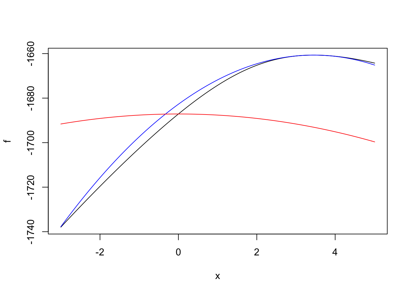
We take a look at Bayesian logistic regression with a fixex prior variance. We compare the performance of adaptive quadrature, Laplace approximation (with expansions around the MLE and MAP), and then Gauss-Hermite quadrature, which ought to refine the Laplace approximation.

A few examples

Code

library(tictoc)
library(dplyr)

Attaching package: 'dplyr'

The following objects are masked from 'package:stats':

    filter, lag

The following objects are masked from 'package:base':

    intersect, setdiff, setequal, union

Code

library(kableExtra)

Attaching package: 'kableExtra'

The following object is masked from 'package:dplyr':

    group_rows

Scenarios: - completely enriched (MLE does not exist, but the LR) - completely separated (\(x=y\), or \(y = 1(x \leq c)\)) - well behaved - c1-66

Code

##### Minimal working example

f <- paste0('', Sys.glob('cache/resources/C1*')) # clear cash so it can knit
if(file.exists(f)){file.remove(f)}

[1] TRUE

Code

make_c1_sim <- function(){
  ##### Minimal working example
  c1 <- gseasusie::load_msigdb_geneset_x('C1')

  # sample random 5k background genes
  set.seed(0)
  background <- sample(rownames(c1$X), 5000)

  # sample GSs to enrich, picked b0 so list is ~ 500 genes
  enriched_gs <- sample(colnames(c1$X), 3)
  b0 <- -2.2
  b <- 3 *abs(rnorm(length(enriched_gs)))
  logit <- b0 + (c1$X[background, enriched_gs] %*% b)[,1]
  y1 <- rbinom(length(logit), 1, 1/(1 + exp(-logit)))
  list1 <- background[y1==1]
  X <- c1$X[background,]
  X <- X[, Matrix::colSums(X) > 1]
  idx <- which(colnames(X) %in% enriched_gs)

  list(X = X, y = y1, idx = idx, b = b, b0 = b0, logits=logit)
}

Code

# "completely enriched"
sim1 <- function(n=500){
  set.seed(1)
  x <- rbinom(n, 1, 0.2)
  y <- rbinom(n, 1, 0.7)
  y[x == 1] = 1
  return(list(x=x, y=y))
}

# "completely separated, binary x"
sim2 <- function(n=500){
  set.seed(2)
  x <- rbinom(n, 1, 0.2)
  y <- x
  return(list(x=x, y=y))
}

# "completely separated, continuous x"
sim3 <- function(n=500){
  set.seed(3)
  x <- rnorm(n)
  y <- as.integer(x > 1.5)
  return(list(x=x, y=y))
}

# "regular simulation, binary x"
sim4 <- function(n=500){
  set.seed(4)
  x <- rbinom(n, 1, 0.2)
  logit <- -1 + x
  prob <- 1/(1 + exp(-logit))
  y <- rbinom(n, 1, prob)
  return(list(x=x, y=y, logit=logit))
}

# "regular simulation, continuous x"
sim5 <- function(n=500){
  set.seed(4)
  x <- rnorm(n)
  logit <- -1 + x
  prob <- 1/(1 + exp(-logit))
  y <- rbinom(n, 1, prob)
  return(list(x=x, y=y, logit=logit))
}

# "c1-GS66 example
sim6 <- function(n=500){
  sim <- make_c1_sim()
  x <- sim$X[,66]
  y <- sim$y
  return(list(x=x, y=y, logit=sim$logits))
}

Code

sim <- sim1()
prior_variance <- 1

compute_log_abf2 <- function(betahat, shat2, lr, prior_variance){
  tau1 <- 1/shat2
  tau0 <- 1/prior_variance
  tau <- tau1 + tau0
  
  lbf <- lr + 0.5 * log(tau1/tau) - 0.5 / (1/tau0 + 1/tau1) * betahat^2
  return(lbf)
}

logsumexp <- function(x){
  C <- max(x)
  return(C + log(sum(exp(x - C))))
}

Diff <- function(f, g){Vectorize(function(b){f(b) - g(b)})}
Exp <- logisticsusie:::Exp
Shift <- logisticsusie:::Shift
Prod <- function(f, g){Vectorize(function(b) f(b) * g(b))}

gauss_hermite <- function(f, mu, tau, ll0, m=16){
  # make quadrature points
  quad_points <- statmod::gauss.quad.prob(
    m, dist='normal', mu=mu, sigma=sqrt(1/tau))
  
  # function logq(b)
  logq <- function(b){
    dnorm(b, mean=mu, sd=sqrt(1/tau), log=T) 
  }
  
  # compute marginal log likelihood
  h <- Diff(f, logq)
  
  # compute log \int f(b)/q(b) q(b) db
  logZ <- logsumexp(h(quad_points$nodes) + log(quad_points$weights))
  lbf <- logZ - ll0
  
  # compute posterior mean
  h1 <- Prod(identity, Exp(Shift(h, logZ)))
  mu <- sum(h1(quad_points$nodes) * quad_points$weights)
  
  h2 <- Prod(function(x){x^2}, Exp(Shift(h, logZ)))
  mu2 <- sum(h2(quad_points$nodes) * quad_points$weights)
  var <- mu2 - mu^2
  
  list(lbf = lbf, logZ = logZ, mu=mu, var=var)
}

driver <- function(sim, prior_variance){
  # 1. mle + laplace
  ll0 <- with(sim, sum(dbinom(y, 1, mean(y), log=T)))
  mle <- with(sim, logisticsusie:::fit_fast_glm(x, y, rep(0, length(y)), ll0))
  mle$lbf <- with(mle, compute_log_abf2(betahat, shat2, lr, prior_variance))
  
  # add approximate posterior to mle
  tau1 <- 1/mle$shat2
  tau0 <- 1/prior_variance
  mle$mu <- tau1/(tau0 + tau1) * mle$betahat
  mle$tau <- tau1 + tau0

  # 2. map + laplace
  map <- with(sim, logisticsusie:::ridge(x, y, prior_variance=1.))
  map$lbf <- with(map, logZ - ll0)
  
  # 3. quadrature
  quad <- with(sim, logisticsusie::logistic_bayes(x, y, prior_variance=1, width=Inf))
  quad$lbf <- quad$logZ - ll0
  
  # 4. setup function
  f <- with(sim, logisticsusie:::make_log_joint(
    x, y, map$intercept, prior_variance))
  g <- logisticsusie:::make_laplace_approx(f, map)
  h <- logisticsusie:::make_laplace_approx(f, mle)

  # 5. Gauss-Hermite centered on MAP
  gh16 <- gauss_hermite(f, map$mu, map$tau, ll0, m=16)
  
  # 6. Gauss-Hermite centered on MLE-approximate MAP
  gh16_mle <- gauss_hermite(f, mle$mu, mle$tau, ll0, m=16)
  
  # 7. plot logp(y, b) and it's MAP and MLE based approximations
  s1 <- 1/sqrt(map$tau)
  range1 <- map$mu + 3* c(-s1, s1)
  
  s2 <- 1/sqrt(mle$tau)
  range2 <- mle$mu + 3* c(-s2, s2)
  
  range <- range(c(range1, range2))
  
  plot(f, xlim = range)
  plot(g,  xlim = range, add=T, col='blue')
  plot(h,  xlim = range, add=T, col='red')
  
  # print(glue::glue('Adaptive = {quad$lbf}\n Laplace(MAP) = {map$lbf}\n Laplace(MLE) = {mle$lbf}\n Gauss-Hermite (MAP, m=16) = {gh16}\n Gauss-Hermite (MLE, m=16) = {gh16_mle}'))
  
  res <- tibble::tribble(
    ~method, ~lbf, ~mu, ~var,
    'Adaptive', quad$lbf, quad$mu, quad$var,
    'Laplace(MAP)', map$lbf, map$mu, 1/map$tau,
    'Laplace(MLE)', mle$lbf, mle$mu, 1/mle$tau,
    'Gauss-Hermite(MAP)', gh16$lbf, gh16$mu, gh16$var,
    'Gauss-Hermite(MLE)', gh16_mle$lbf, gh16_mle$mu, gh16_mle$var
  )
  return(res)
}

Completely enriched

Code

res1 <- driver(sim1(), prior_variance=1)

Code

res1 %>%
  kableExtra::kable(digits=2)

method	lbf	mu	var
Adaptive	25.14	2.83	0.28
Laplace(MAP)	25.13	2.74	0.27
Laplace(MLE)	25.84	0.00	1.00
Gauss-Hermite(MAP)	25.14	2.83	-0.25
Gauss-Hermite(MLE)	25.14	2.83	-7.78

Completely separated, binary \(x\)

Code

res2 <- driver(sim2(), prior_variance=1)

Code

res2 %>%
  kableExtra::kable(digits=2)

method	lbf	mu	var
Adaptive	223.33	6.80	0.14
Laplace(MAP)	223.33	6.75	0.14
Laplace(MLE)	249.34	0.00	1.00
Gauss-Hermite(MAP)	223.33	6.80	-0.57
Gauss-Hermite(MLE)	223.63	6.63	-43.97

Completely separated, continuous \(x\)

Code

res3 <- driver(sim3(), prior_variance=1)

Warning: fit_glm: fitted probabilities numerically 0 or 1 occurred

Code

res3 %>%
  kableExtra::kable(digits=2)

method	lbf	mu	var
Adaptive	117.09	4.90	0.03
Laplace(MAP)	117.09	4.89	0.03
Laplace(MLE)	139.34	0.00	1.00
Gauss-Hermite(MAP)	117.09	4.90	-0.01
Gauss-Hermite(MLE)	115.43	4.60	-21.14

Regular simulation, binary \(x\)

Code

res4 <- driver(sim4(n=500), prior_variance=1)

Code

res4 %>%
  kableExtra::kable(digits=2)

method	lbf	mu	var
Adaptive	10.24	1.08	0.04
Laplace(MAP)	10.24	1.08	0.04
Laplace(MLE)	11.88	1.08	0.05
Gauss-Hermite(MAP)	10.24	1.08	0.04
Gauss-Hermite(MLE)	10.24	1.08	0.04

Regular simulation, continuous \(x\)

Code

res5 <- driver(sim4(n=500), prior_variance=1)

Code

res5 %>%
  kableExtra::kable(digits=2)

method	lbf	mu	var
Adaptive	10.24	1.08	0.04
Laplace(MAP)	10.24	1.08	0.04
Laplace(MLE)	11.88	1.08	0.05
Gauss-Hermite(MAP)	10.24	1.08	0.04
Gauss-Hermite(MLE)	10.24	1.08	0.04

C1 Example

Code

res6 <- driver(sim6(), prior_variance=1)

loading gene set from msigdbr: C1

Adding missing grouping variables: `geneSet`

Code

res6 %>%
  kableExtra::kable(digits=2)

method	lbf	mu	var
Adaptive	25.69	3.51	0.28
Laplace(MAP)	25.68	3.45	0.27
Laplace(MLE)	30.79	0.00	1.00
Gauss-Hermite(MAP)	25.69	3.51	-0.12
Gauss-Hermite(MLE)	25.69	3.51	-12.24