Wakefield ABF Accuracy

We noticed that the error in Wakefield’s ABF grows with increasing sample size. This is surprising, because at these large sample sizes asymptotic normality kicks in. The issue can be more clearly seen by considering the ABF as an integral over an approximation to the likelihood ratio. The approximation used in the ABF ensure that the approximate likelihood ratio at \(0\) is 1, but that the curvature and mode of the approximation are determined by the asymptotic distribution of the MLE. This leads to a gap in the approximate likelihood ratio and the exact likelihood ratio around the mode. As the normal approximation becomes more peaked, the accuracy of the ABF is increasingly determined by the quality of the likelihood ratio approximation in a small neighborhood around the mode which is off by this gap, which appears to grow with sample size.

Author

Karl Tayeb

Published

April 25, 2023

Code

library(dplyr)
library(ggplot2)

sigmoid <- function(x){1/(1 + exp(-x))}

simulate <- function(n, beta0=0, beta=1){
  x <- rnorm(n)
  logit <- beta0 + beta*x
  y <- rbinom(n, 1, sigmoid(logit))
  return(list(x=x, y=y, beta0=beta0, beta=beta))
}

fit_glm_no_intercept <- function(sim){
  fit <- with(sim, glm(y ~ x + 0, family = 'binomial'))
  tmp <- unname(summary(fit)$coef[1,])
  betahat <- tmp[1]
  shat2 <- tmp[2]^2
  z <- with(sim, (beta - betahat)/sqrt(shat2))
  res <- list(
    intercept=0,
    betahat = betahat,
    shat2 = shat2,
    z = z
  )
  return(res)
}

fit_glm <- function(sim, prior_variance=1){
  fit <- with(sim, glm(y ~ x + 1, family = 'binomial'))
  tmp <- unname(summary(fit)$coef[2,])
  betahat <- tmp[1]
  shat2 <- tmp[2]^2
  z <- with(sim, (beta - betahat)/sqrt(shat2))
  res <- list(
    intercept = unname(fit$coefficients[1]),
    betahat = betahat,
    shat2 = shat2,
    z = z
  )
  return(res)
}

compute_log_abf1 <- function(betahat, shat2, prior_variance){
  W <- prior_variance
  V <- shat2
  z <- betahat / sqrt(shat2)
  labf <- 0.5 * log(V /(V + W)) + 0.5 * z^2 * W /(V + W)
  return(labf)
}

compute_log_abf2 <- function(betahat, shat2, prior_variance){
  dnorm(betahat, 0, sqrt(shat2 + prior_variance), log = T) - 
    dnorm(betahat, 0, sqrt(shat2), log=T)
}

compute_log_abf <- function(glm_summary, prior_variance=1){
  labf <- with(glm_summary, compute_log_abf1(betahat, shat2, prior_variance))
  return(labf)
}

compute_exact_log_abf_no_intercept <- function(sim, prior_variance){
  glm_fit <- fit_glm_no_intercept(sim)
  f <- function(b){
    logits <- sim$x * b
    sum(dbinom(x=sim$y, size=1, prob=sigmoid(logits), log = T)) + 
      dnorm(b, 0, sqrt(prior_variance), log = T)
  }
  max <- f(glm_fit$betahat)
  
  f2 <- function(b){purrr::map_dbl(b, ~exp(f(.x) - max))}
  
  lower <- glm_fit$betahat - sqrt(glm_fit$shat2) * 6
  upper <- glm_fit$betahat + sqrt(glm_fit$shat2) * 6
  quadres <- cubature::pcubature(f2, lower, upper, tol = 1e-10)
  log_bf <- (log(quadres$integral) + max) - sum(dbinom(sim$y, 1, 0.5, log=T))
  return(log_bf)
}

compute_exact_log_bf <- function(sim, prior_variance){
  glm_fit <- fit_glm(sim)
  f <- function(b){
    logits <- sim$x * b + glm_fit$intercept
    sum(dbinom(x=sim$y, size=1, prob=sigmoid(logits), log = T)) + 
      dnorm(b, 0, sqrt(prior_variance), log = T)
  }
  max <- f(glm_fit$betahat)
  
  f2 <- function(b){purrr::map_dbl(b, ~exp(f(.x) - max))}
  
  lower <- glm_fit$betahat - sqrt(glm_fit$shat2) * 6
  upper <- glm_fit$betahat + sqrt(glm_fit$shat2) * 6
  quadres <- cubature::pcubature(f2, lower, upper, tol = 1e-10)
  log_bf <- (log(quadres$integral) + max) - sum(dbinom(sim$y, 1, mean(sim$y), log=T))
  return(log_bf)
}

compute_vb_log_bf <- function(sim, prior_variance=1){
  vb <- with(sim, logisticsusie::fit_univariate_vb(x, y, tau0=1/prior_variance)) 
  log_vb_bf <- tail(vb$elbos, 1) - sum(dbinom(sim$y, 1, mean(sim$y), log=T))
  return(log_vb_bf)
}

Code

# compute ABF, variational BF, and exact BF via quadrature
bf_comparison <- function(...){
  sim <- simulate(...)
  a <- sim %>% fit_glm() %>% compute_log_abf(prior_variance=1)
  b <- sim %>% compute_vb_log_bf(prior_variance=1)
  c <- sim %>% compute_exact_log_bf(prior_variance=1)
  tibble(log_abf = a, log_vbf = b, log_bf = c)
}

bf_comparison_rep <- function(reps, n, beta){
  purrr::map_dfr(1:reps, ~bf_comparison(n=n, beta=beta)) %>% mutate(n=n, beta=beta, rep=1:reps)
}

# scale_log2x <- scale_x_continuous(trans = log2_trans(),
#     breaks = trans_breaks("log2", function(x) 2^x),
#     labels = trans_format("log2", math_format(2^.x)))

Demonstrations

Here we simulate \(x_i \sim N(0, 1)\) and \(y_i \sim \text{Bernoulli}(\sigma(x_i \beta + \beta_0))\)

\(\beta = 0.1\), \(\beta_0 = 0\)

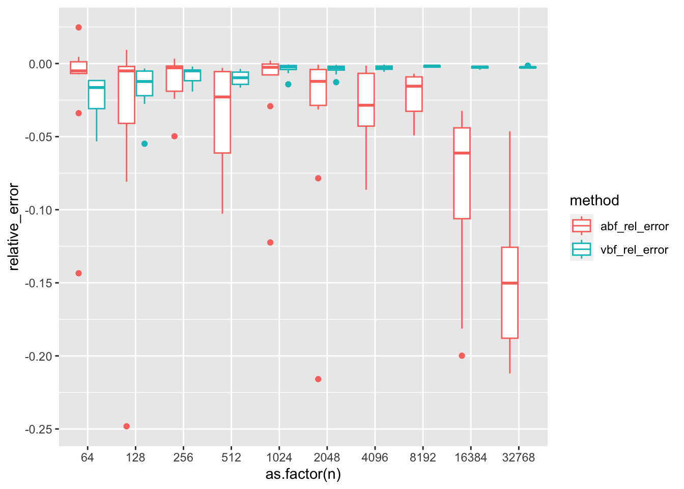
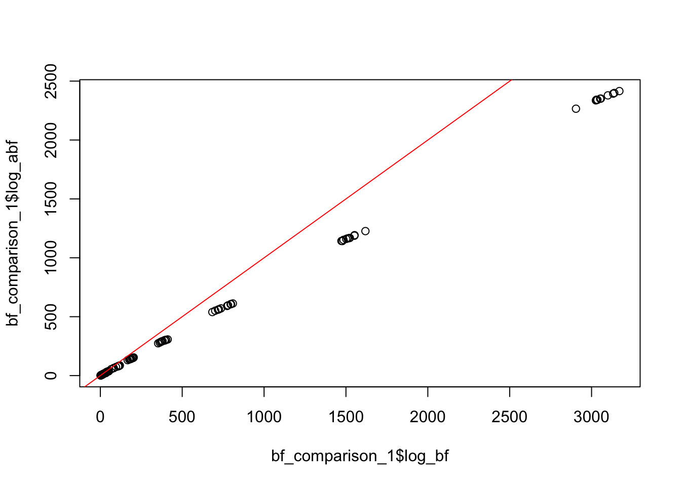
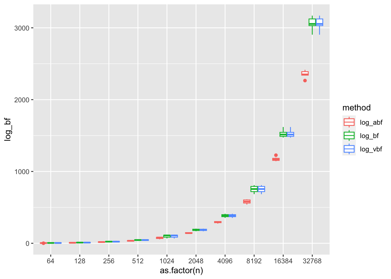
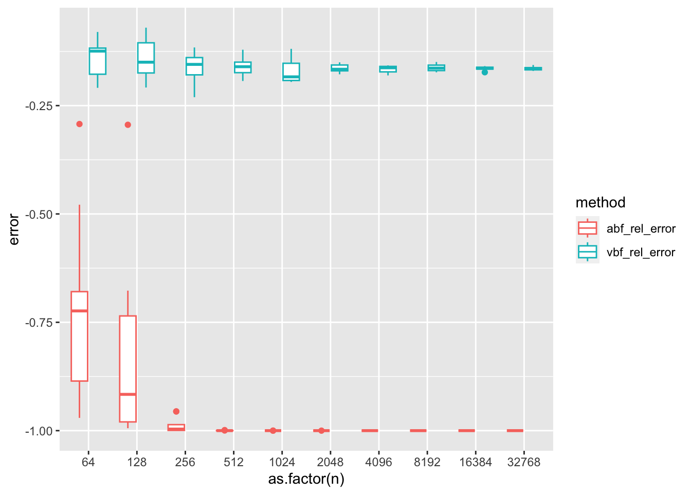
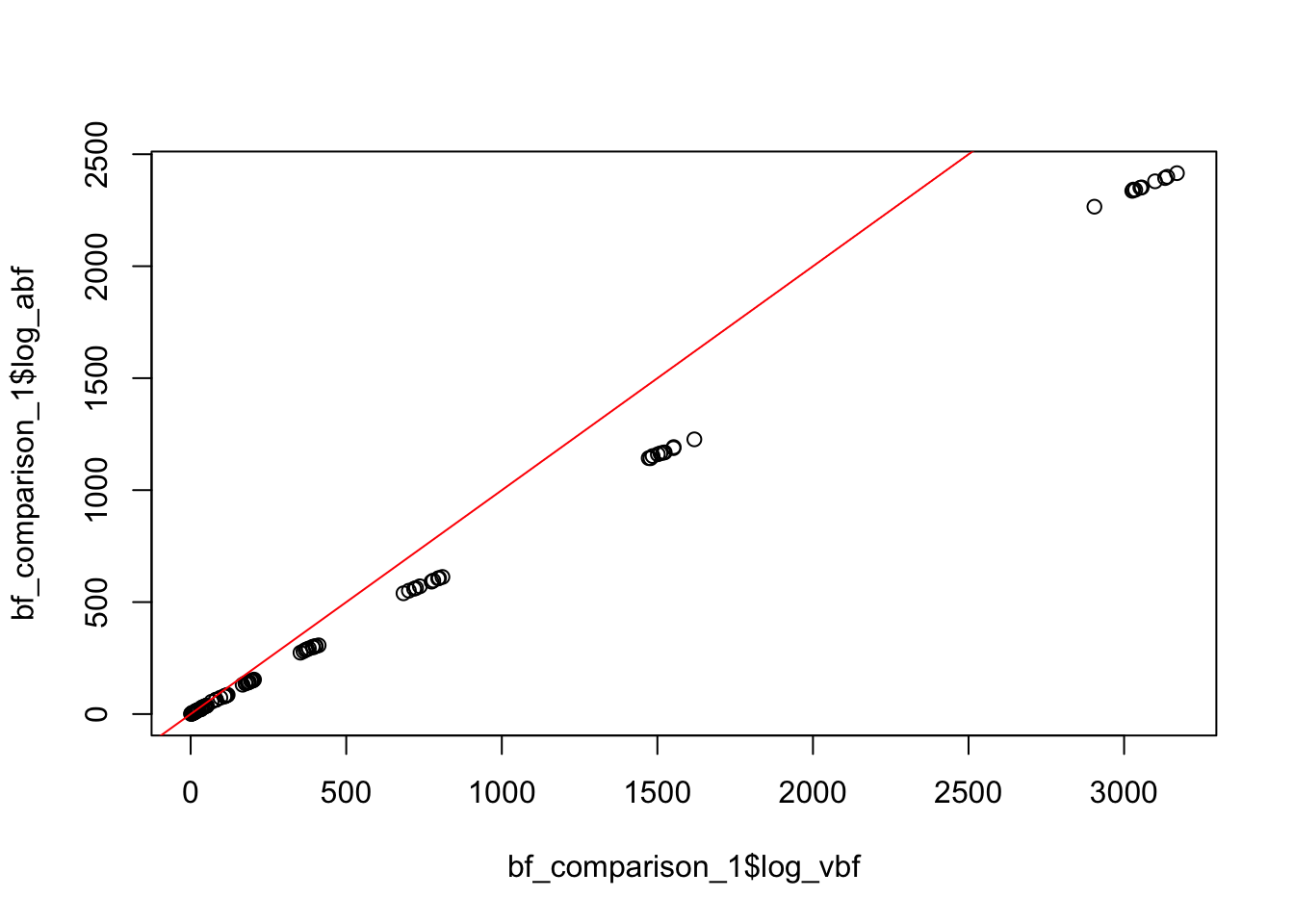
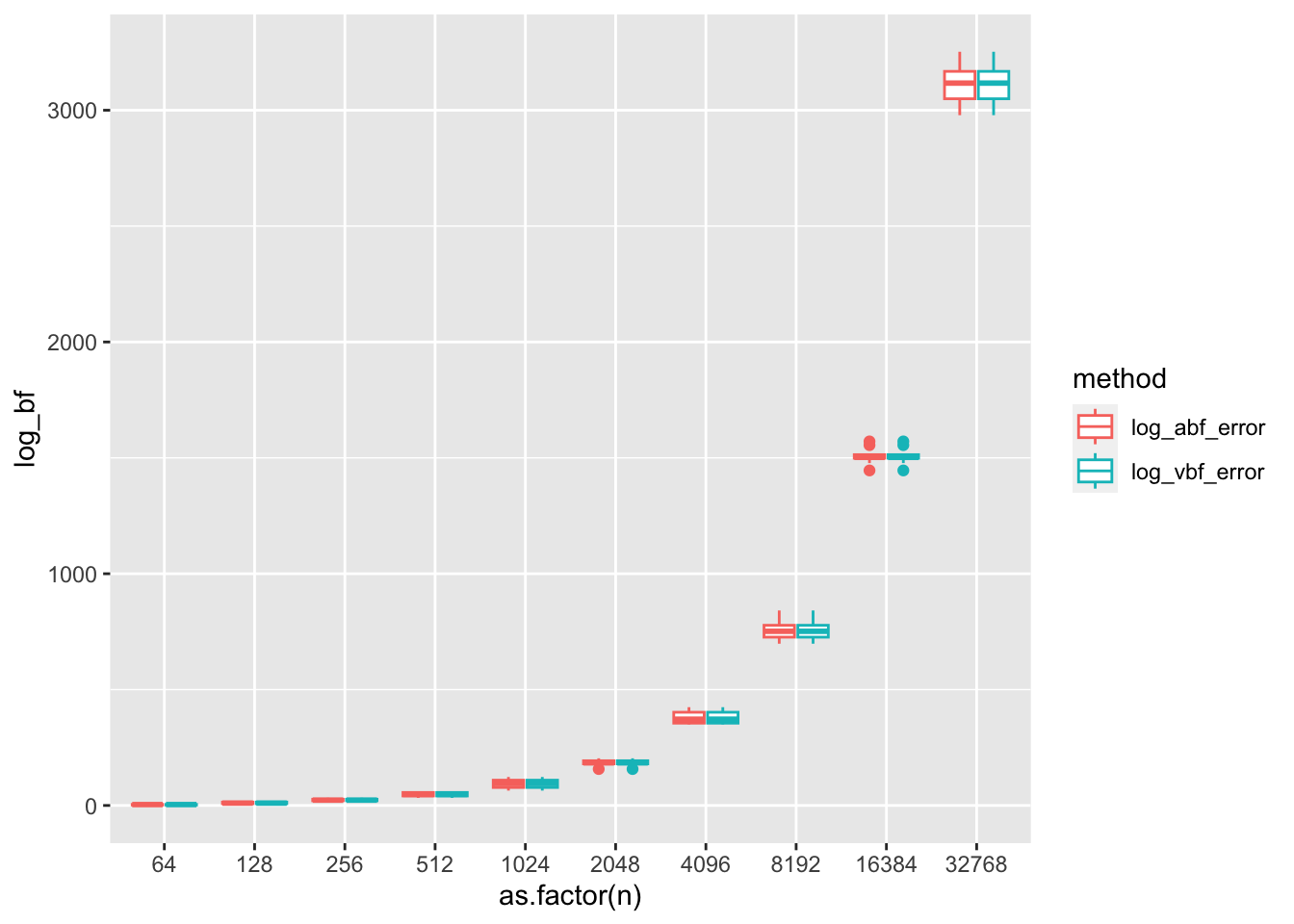
We simulate 10 replications at each sample size \(n = 2^6, 2^7, \dots, 2^{16}\). While we see relatively good agreement between the ABF and exact BF on a log-scale, we do see the pattern that the error tends to increase with increasing samples size. Furthermore, these “small” errors on the log scale actually translate to large errors between the BF and ABF.

Code

# range of n, 10 reps
n <- 2^(6:15)
bf_comparison_01 <- purrr::map_dfr(n, ~bf_comparison_rep(10, .x, 0.1))

# "good" agreement the exact BF and ABF
par(mfrow=c(1, 2))
plot(bf_comparison_01$log_bf,
     bf_comparison_01$log_abf,
     xlab='log BF', ylab = 'log ABF'); abline(0, 1, col='red')
plot(bf_comparison_01$log_bf,
     bf_comparison_01$log_abf - bf_comparison_01$log_bf,
     xlab = 'log BF', ylab = 'log ABF - log BF'); abline(h=0, col='red')

Code

# bf_comparison_01 %>% 
#   tidyr::pivot_longer(ends_with('bf'), names_to='method', values_to='log_bf') %>%
#   ggplot(aes(x=as.factor(n), y=log_bf, color=method)) +
#   geom_boxplot()


bf_comparison_01 %>% 
  mutate(
    abf_rel_error = exp(log_abf - log_bf) - 1,
    vbf_rel_error = exp(log_vbf - log_bf) - 1) %>%
  tidyr::pivot_longer(ends_with('error'), names_to='method', values_to='relative_error') %>%
  ggplot(aes(x=as.factor(n), y=relative_error, color=method)) +
  geom_boxplot()

Surprisingly as \(n\) grows, the relative error between the BF and the ABF increases! At \(n=2^9\) things look pretty good, but at \(n=2^15\) the relative error is quite large! Let’s inspect the \(z\)-scores at these simulation settings– do they look normally distributed?

Confirming normality

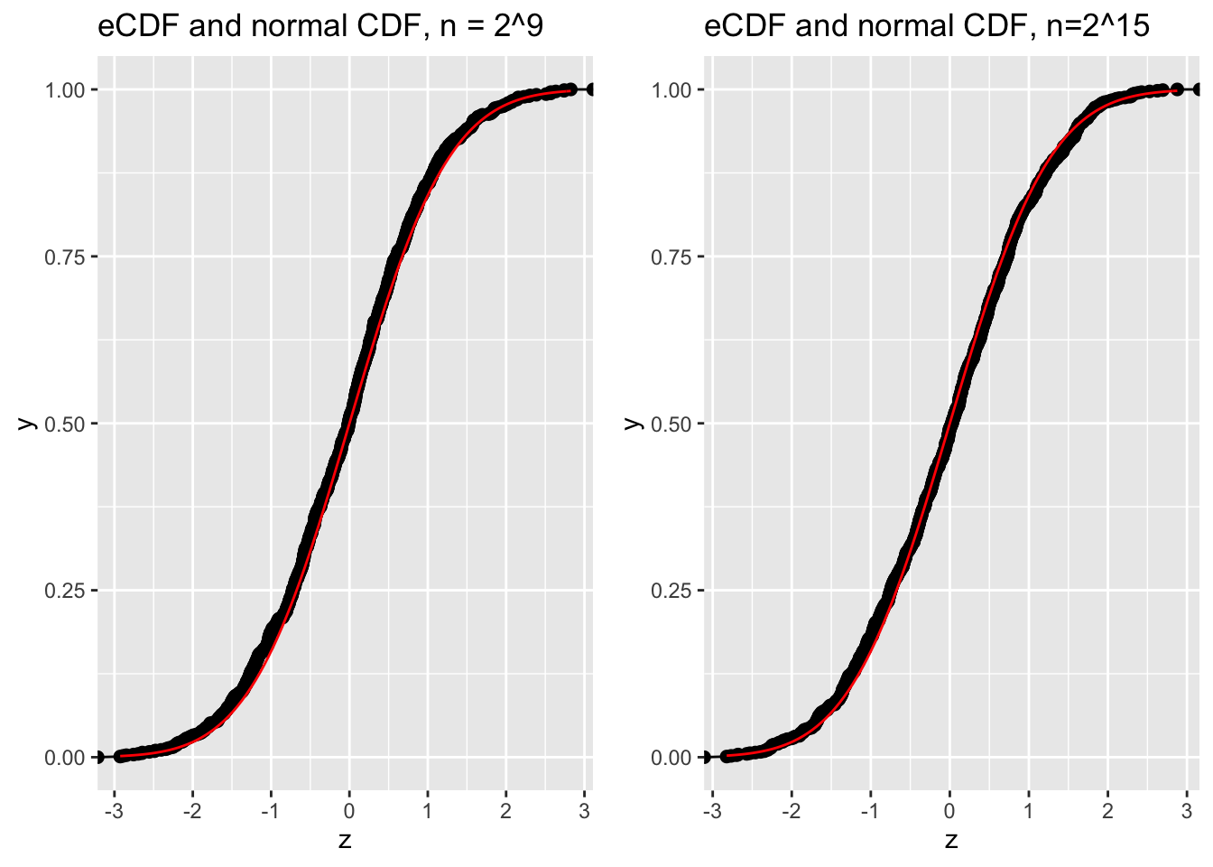
Both \(n=2^9\) and \(n=2^{15}\) are fairly large sample sizes. We confirm that \(z = \frac{\beta - \hat\beta}{\hat s}\) looks normal

Code

glm_sim_reps <- function(reps, n, beta){
  purrr::map_dfr(1:reps, ~simulate(n, beta=beta) %>% fit_glm() %>% data.frame()) %>%
    mutate(rep = 1:reps)
}

rep1 <- glm_sim_reps(1000, 2^9, 0.1)
shapiro.test(rep1$z)


    Shapiro-Wilk normality test

data:  rep1$z
W = 0.99826, p-value = 0.4108

Code

ks.test(rep1$z, pnorm)


    One-sample Kolmogorov-Smirnov test

data:  rep1$z
D = 0.030303, p-value = 0.3175
alternative hypothesis: two-sided

Code

rep2 <- glm_sim_reps(1000, 2^15, 0.1)
shapiro.test(rep2$z)


    Shapiro-Wilk normality test

data:  rep2$z
W = 0.99693, p-value = 0.05116

Code

ks.test(rep2$z, pnorm)


    One-sample Kolmogorov-Smirnov test

data:  rep2$z
D = 0.027911, p-value = 0.4172
alternative hypothesis: two-sided

Code

p1 <- ggplot(rep1,aes(x=z)) +
       geom_line(stat = "ecdf")+
       geom_point(stat="ecdf",size=2) +
       stat_function(fun=pnorm,color="red") +
       labs(title="eCDF and normal CDF, n = 2^9")
p2 <- ggplot(rep2,aes(x=z)) +
       geom_line(stat = "ecdf")+
       geom_point(stat="ecdf",size=2) +
       stat_function(fun=pnorm,color="red") +
       labs(title="eCDF and normal CDF, n=2^15")

cowplot::plot_grid(p1, p2)

Code

subset_sim <- function(sim, m){
  sim2 <- sim
  sim2$x <- head(sim2$x, m)
  sim2$y <- head(sim2$y, m)
  return(sim2)
}

beta <- 0.1
sim <- simulate(2^16, beta=beta)
titrate <- purrr::map_dfr(5:16, ~sim %>% subset_sim(2^.x) %>% fit_glm() %>% data.frame())
plotrix::plotCI(
  x= 5:16,
  y= titrate$betahat - beta,
  li = (titrate$betahat - beta) - 2 * sqrt(titrate$shat2),
  ui = (titrate$betahat - beta) + 2 * sqrt(titrate$shat2)
); abline(h=0, lty=3)

I was wondering if glm applies a conservative correction to it’s estimate of the standard error. The standard errors come from the squareroot of the diagonal of the negative inverse Fisher information matrix since asymptotically.

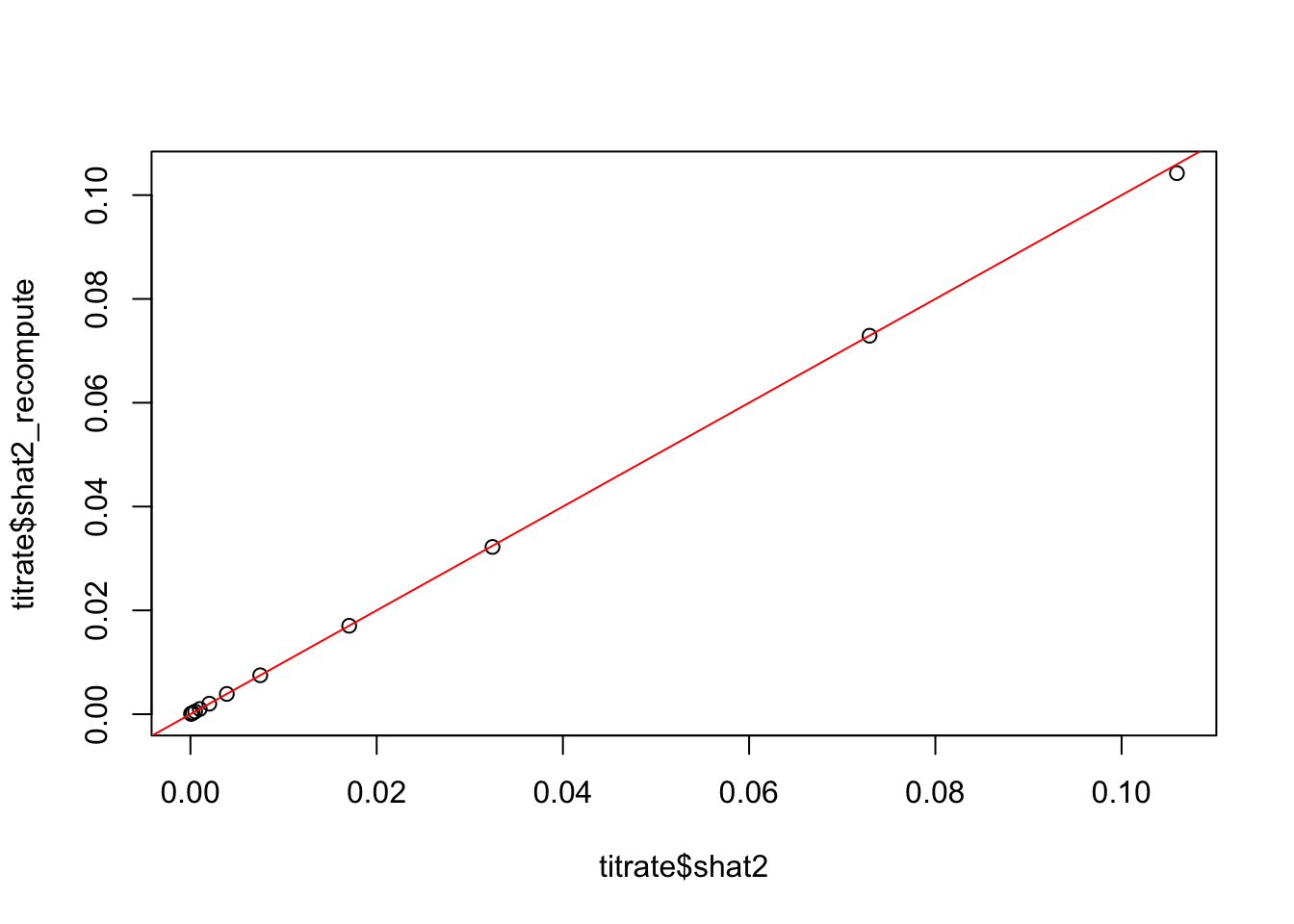
\[ \hat \beta \sim N(\beta, - \mathcal I(\beta)^{-1}) \] I think peoples use \(- \mathcal I(\hat \beta)\) as an estimator for the precision matrix. Ignoring the intercept I just computed \(I = \sum_i \nabla^2_{\beta}\log p (y |x, \beta, \beta_0)\), and used \(s_2 = \sqrt{I^{-1}}\) as a new estimate of the standard error. Despite some hadn waiving, it actually agrees very well with the standard errors reported by glm– which is to say this is not the problem.

Code

recompute_shat2 <- function(betahat, intercept, x){
  logits <- betahat * x + intercept
  return(1/sum(sigmoid(logits) * sigmoid(-logits) * x^2))
}

titrate <- titrate %>%
  mutate(m = 2^(5:16)) %>%
  rowwise() %>%
  mutate(shat2_recompute = recompute_shat2(betahat, intercept, head(sim$x, m))) %>%
  ungroup()

plot(titrate$shat2, titrate$shat2_recompute); abline(0, 1, col='red')

\(\beta = 1\)

For larger \(\beta\) the discrepency between ABF and BF is much more obvious!

Code

n <- 2^(6:15)
bf_comparison_1 <- purrr::map_dfr(n, ~bf_comparison_rep(10, .x, 1))

plot(bf_comparison_1$log_bf, bf_comparison_1$log_abf); abline(0, 1, col='red')

Code

bf_comparison_1 %>% 
  tidyr::pivot_longer(ends_with('bf'), names_to='method', values_to='log_bf') %>%
  ggplot(aes(x=as.factor(n), y=log_bf, color=method)) +
  geom_boxplot()

Code

bf_comparison_1 %>% 
  mutate(
    abf_rel_error = exp(log_abf - log_bf) - 1,
    vbf_rel_error = exp(log_vbf - log_bf) - 1) %>%
  tidyr::pivot_longer(ends_with('error'), names_to='method', values_to='error') %>%
  ggplot(aes(x=as.factor(n), y=error, color=method)) +
  geom_boxplot()

Code

plot(bf_comparison_1$log_vbf, bf_comparison_1$log_abf);abline(0, 1, col='red')

Code

n <- 2^(6:15)
bf_comparison_01 <- purrr::map_dfr(n, ~bf_comparison_rep(10, .x, 1))
bf_comparison_01 %>% 
  mutate(log_abf_error = (log_abf - log_bf), log_vbf_error = (log_vbf - log_bf)) %>%
  tidyr::pivot_longer(ends_with('error'), names_to='method', values_to='error') %>%
  ggplot(aes(x=as.factor(n), y=log_bf, color=method)) +
  geom_boxplot()

An explaination

\[ \begin{aligned} ABF &= \int \frac{N(\hat \beta| \beta, s^2)}{N(\hat\beta | 0, s^2)} p(\beta) d\beta\\ BF &= \int \frac{p({\bf y} | {\bf x}, \beta)}{p({\bf y} | \beta = 0)} p(\beta) d\beta \end{aligned} \]

First, here is an example where there is a large discrepancy between the log ABF and log BF– over 20 log-likelihood units! We also note that including/excluding the intercept in glm doesn’t really make a dent.

Code

set.seed(2)
sim <- simulate(1000)
fit <- fit_glm(sim, prior_variance=1)
fit_no_intercept <- fit_glm_no_intercept(sim)

# show there is a discrepency ~20 log-likelihood unit
with(fit, compute_log_abf1(betahat, shat2, 1))

[1] 71.33497

Code

with(fit_no_intercept, compute_log_abf1(betahat, shat2, 1))

[1] 71.46433

Code

compute_vb_log_bf(sim, 1)

[1] 93.52508

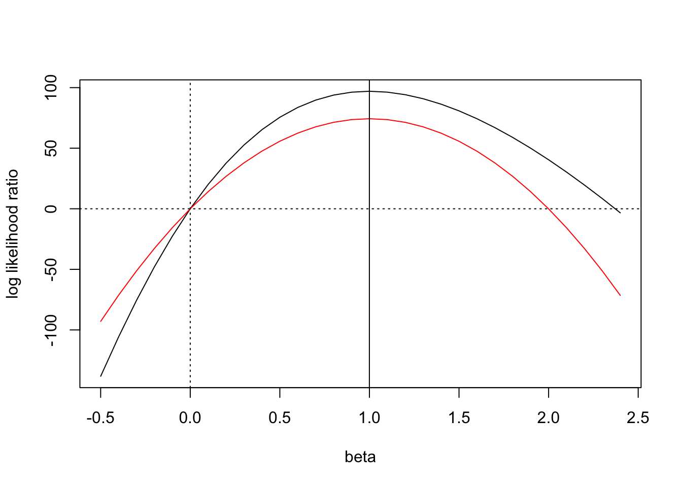
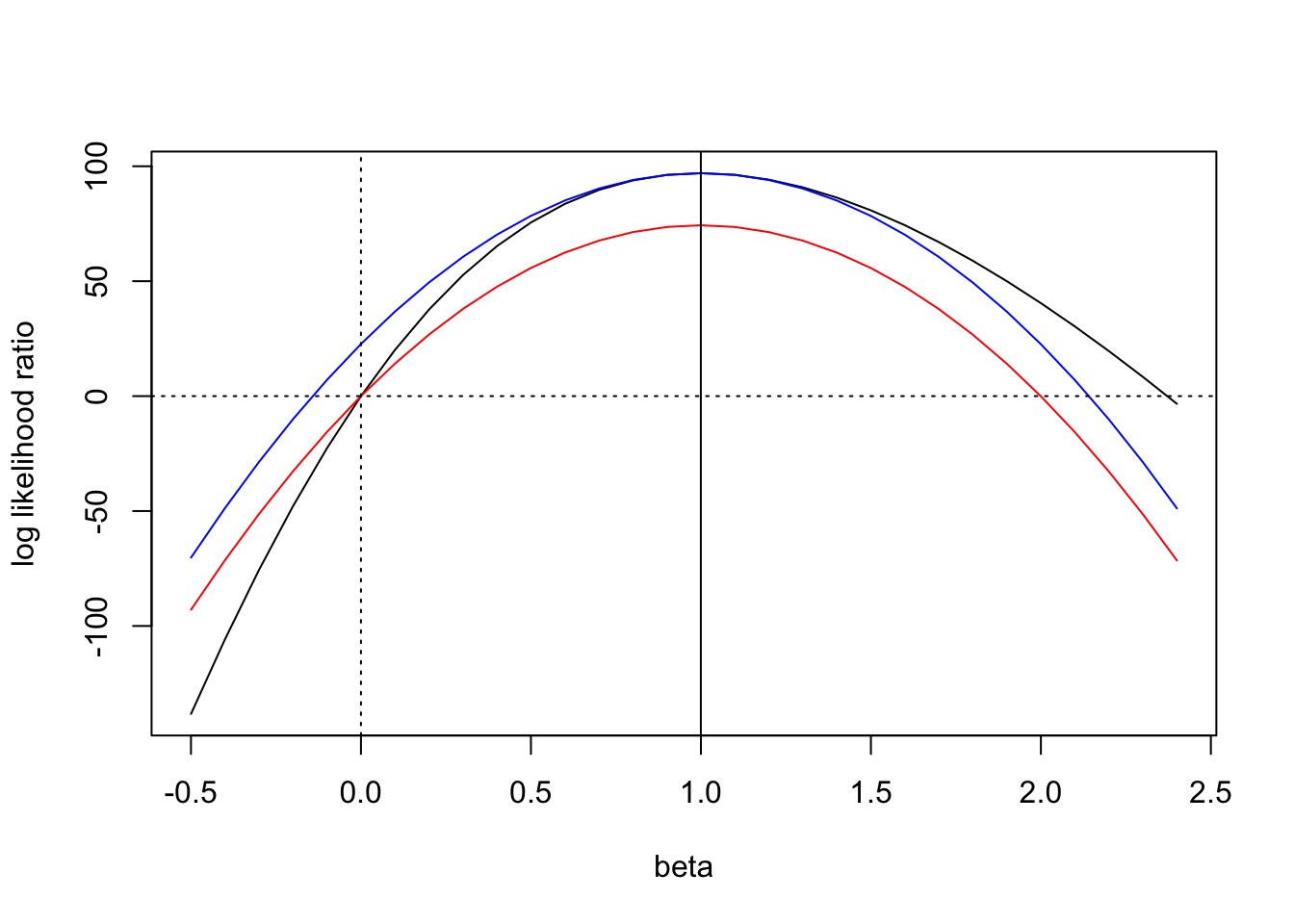
Using this simulated example we plot the likelihood ratio and approximate log-likelihood ratio (with respect to the null model \(\beta=0\)) over the range of \(\beta\). We plot the likelihood ratio in black, and plot the approximate likelihood ratio in red. We see that the likelihood ratios agree at \(\beta = 0\)– this is not surprising because they should both be equal to \(1\) (or \(0\), on the log scale as shown in the plot).

The mode and the curvature of this likelihood ratio approximation are determined by the effect size and standard error, so the approximation is completely specified. We can see that this leaves a gap between the likelihood ratio and the approximate likelihood ratio near the mode. Assuming a flat prior on \(\beta\), this is the region that will contribute most to the integral.

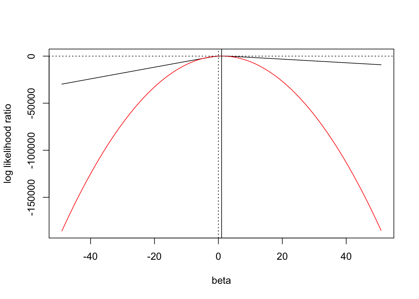
While the likelihood is well approximated by a Gaussian near it’s mode, the quality of the Gaussian approximation is poor in the tails. As the sample size increases, \(\beta = 0\) is more “in the tail”. So we see that the approximation to the likelihood ratio used in ABF is requiring the approximate likelihood ratio to agree with the exact likelihood ratio at some point in the tail– but this is not particularly relevant for getting a good approximation of the BF, as it is the area in the body of the distribution that contributes most to the integral.

In order for the ABF to perform well in large samples, the Gaussian approximation would need to improve in the tails faster than the point \(\beta=0\) gets pushed into the tail. E.g. for the Gaussian approximation to be good, we’d want that the curvature estimated at the mode is also the curvature we’d estimate everywhere else (e.g. at \(\beta = 0\)).

Code

compare_lrs <- function(sim, prior_variance=1, k=1, plot_correction=F){
  fit <- fit_glm(sim, prior_variance=1)
  fit_no_intercept <- fit_glm_no_intercept(sim)
  
  # plot ll
  ll <- function(b){with(sim, sum(y*x*b - log(1 + exp(x*b))))}
  ll_vec <- function(b){purrr::map_dbl(b, ~ll(.x))}
  asymptotic_ll <- function(b){dnorm(b, mean=fit$betahat, sd=sqrt(fit$shat2), log=T)}

  ll0 <- ll(0)
  asymptotic_ll0 <- asymptotic_ll(0)
  
  ll_mle <- ll(fit$betahat)
  asymptotic_ll_mle <- asymptotic_ll(fit$betahat)
  
  mle = fit$betahat
  xs <- seq(mle - k* abs(mle), mle + k* abs(mle), by=0.1)
  
  diff = (ll_mle - asymptotic_ll_mle) - ll0
  ll_xs <- ll_vec(xs)
  asymptotic_ll_xs <- asymptotic_ll(xs)
  ll_prior <- dnorm(xs, 0, sd = sqrt(prior_variance), log = T)
  
  ylim <- range(asymptotic_ll_xs - asymptotic_ll0, ll_xs - ll0)
  plot(xs,ll_xs - ll0, type='l', ylim = ylim,
       xlab= 'beta', ylab='log likelihood ratio')
  lines(xs, asymptotic_ll_xs - asymptotic_ll0, col='red')
  
  if(plot_correction){
    lines(xs, asymptotic_ll_xs - asymptotic_ll_mle + (ll_mle - ll0), col='blue')
  }
  abline(h=0, lty=3)
  abline(v=0, lty=3)
  abline(v=fit$betahat)
}

compare_lrs(sim, prior_variance = 1, k=1.5)

Code

compare_lrs(sim, prior_variance = 1, k=50)

Code

par(mfrow=c(1, 4))
simulate(100, beta0 = 0.1) %>% compare_lrs(k=1.5)
simulate(1000, beta0 = 0.1) %>% compare_lrs(k=1.5)
simulate(10000, beta0 = 0.1) %>% compare_lrs(k=1.5)
simulate(100000, beta0 = 0.1) %>% compare_lrs(k=1.5)

Family of LR approximations

Write the likelihood ratio as \[ LR(\beta_1, \beta_2) = \frac{\mathcal {L}(\beta_1)}{\mathcal {L}(\beta_2)} \]

Let \(\widehat {LR}(\beta_1, \beta_2)\) be the approximate likelihood ratio under the normal approximation \(\beta \sim N(\hat \beta, s^2)\).

The approximation to the likelihood ratio against the null used in ABF is simply

\[ \widehat{LR}_{ABF}(\beta) = \widehat{LR}(\beta, 0) \] However if we note that

\[ LR(\beta, 0) = LR(\beta, \beta^*) \times LR(\beta^*, 0) \]

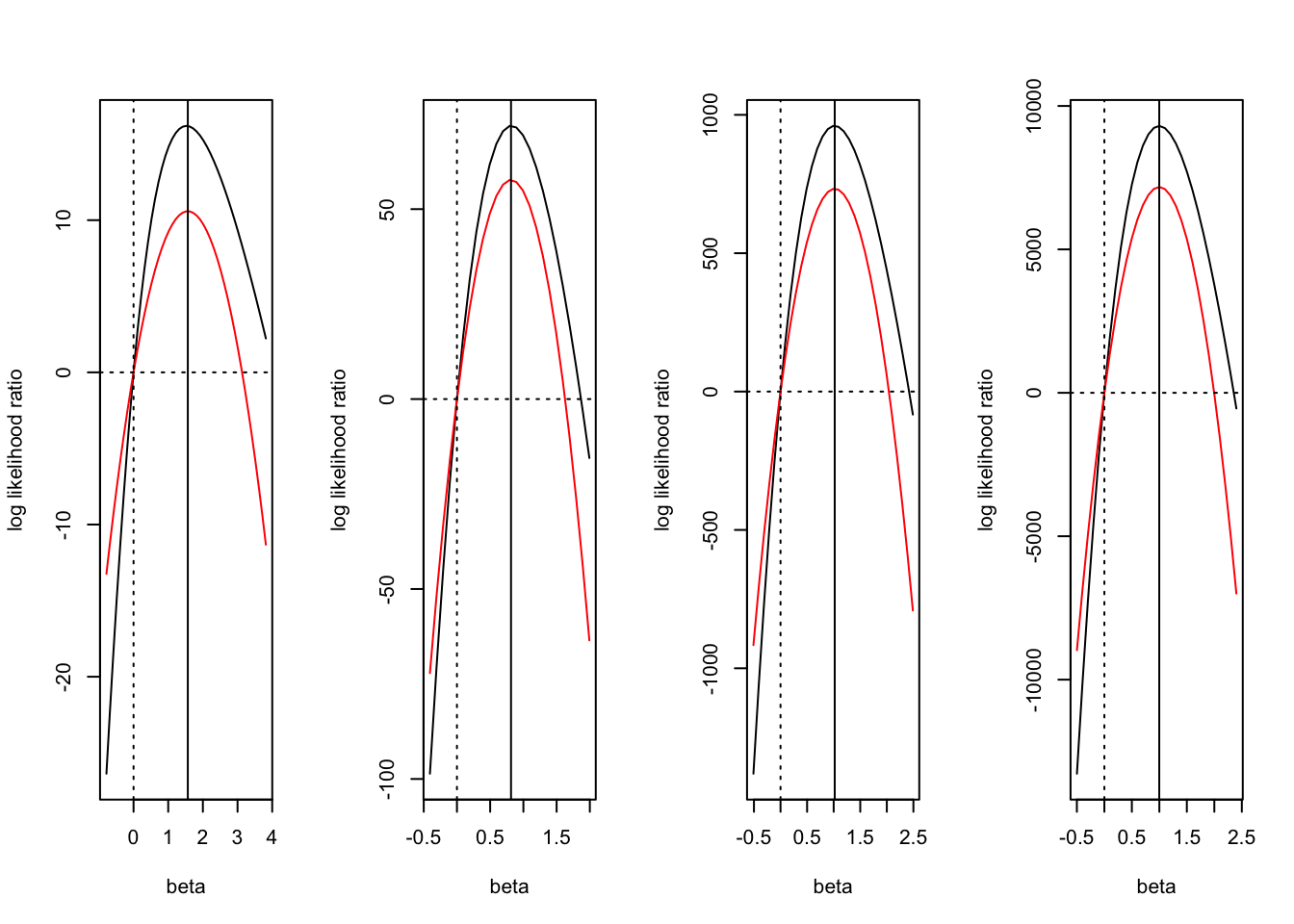
we can derive a family of approximations for the likelihood ratio against the null

\[ \widehat{LR}_{\beta^*}(\beta) = \widehat{LR}(\beta, \beta^*) LR(\beta^*,0) \] And note that \(\widehat{LR}_{ABF}\) is a special case where \(\beta^*=0\). We’ve seen that this choice makes the approximation good in the tail– which isn’t very important for getting an accurate approximate BF. Perhaps the best choice would be make the approximate LR match the exact LR at the MAP estimate. But a second good choice, and one that does not require knowledge of the prior could be to set \(\beta^* = \beta_{MLE}\). This choice is shown in blue on the updated plot

Code

compare_lrs(sim, prior_variance = 1, k=1.5, plot_correction=T)

We can use the