Minimal working example for GSEA SuSiE

This was supposed to be a minimal working example, but when Matthew ran it he got different results than me. When I ran it again this morning I got results that agreed with his. So now this document is meant to diagnose what went wrong!

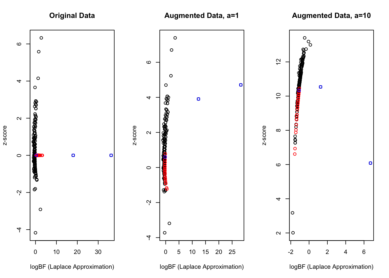
The MLE for the univariate doesn’t exist when the observations. When \(X\) is binary (e.g. in GSEA) if all of the genes in the gene set are in the gene list we can always improve the likelihood by increasing the effect size. Similarly if none of the genes in the gene set are in the gene list, we can always improve the likelihood by decreasing the effect size. When we fit the GLM in these cases using fastglm it will return a large effect size (e.g. \(\hat \beta = 14\)) and very large standard error \(\hat s \approx 20,000\). Consequently we get a \(z\)-score close to zero, but the reported likelihood ratio (LR) can be very large, and may depends on the stopping criteria from the GLM fitting procedure. Also note that when \(y_i = 0 \;\forall i \text{ s.t. } x_i=0\) the data are completely separable and the LR becomes unbounded. However, more often in our setting we will have that there is a limiting value for the LR given by the likelihood of the data in the intercept only model excluding the data where \(x_i=1\) and including the observations where \(x_i = 1\) (I thinks this is correct, but I need to check).

Failing example

Code

library(tictoc)

# devtools::install_github('karltayeb/logisticsusie')
# devtools::install_github('karltayeb/gseasusie')

##### Minimal working example

f <- paste0('', Sys.glob('cache/resources/C1*')) # clear cash so it can knit
if(file.exists(f)){file.remove(f)}

[1] TRUE

Code

make_c1_sim <- function(){
  ##### Minimal working example
  c1 <- gseasusie::load_msigdb_geneset_x('C1')

  # sample random 5k background genes
  set.seed(0)
  background <- sample(rownames(c1$X), 5000)

  # sample GSs to enrich, picked b0 so list is ~ 500 genes
  enriched_gs <- sample(colnames(c1$X), 3)
  b0 <- -2.2
  b <- 3 *abs(rnorm(length(enriched_gs)))
  logit <- b0 + (c1$X[background, enriched_gs] %*% b)[,1]
  y1 <- rbinom(length(logit), 1, 1/(1 + exp(-logit)))
  list1 <- background[y1==1]
  X <- c1$X[background,]
  X <- X[, Matrix::colSums(X) > 1]
  idx <- which(colnames(X) %in% enriched_gs)

  list(X = X, y = y1, idx = idx, b = b, b0 = b0, logits=logit)
}

sim <- make_c1_sim()

loading gene set from msigdbr: C1

Adding missing grouping variables: `geneSet`

Code

X <- sim$X
y <- sim$y
y1 <- y

Code

# GIBSS fit
tic()
fit <- logisticsusie::generalized_ibss(X, y, L=10, estimate_prior_variance = F, maxit=10)

46.176 sec elapsed

Code

toc()

46.191 sec elapsed

Code

fit$prior_variance

 L1  L2  L3  L4  L5  L6  L7  L8  L9 L10 
  1   1   1   1   1   1   1   1   1   1 

Code

fit$cs

$L1
CS = {66} 
 alpha = {1} 
 size = 1, coverage = 1, requested = 0.95
$L2
CS = {66} 
 alpha = {1} 
 size = 1, coverage = 1, requested = 0.95
$L3
CS = {66} 
 alpha = {1} 
 size = 1, coverage = 1, requested = 0.95
$L4
CS = {66} 
 alpha = {1} 
 size = 1, coverage = 1, requested = 0.95
$L5
CS = {66} 
 alpha = {1} 
 size = 1, coverage = 1, requested = 0.95
$L6
CS = {66} 
 alpha = {1} 
 size = 1, coverage = 1, requested = 0.95
$L7
CS = {66} 
 alpha = {1} 
 size = 1, coverage = 1, requested = 0.95
$L8
CS = {66} 
 alpha = {1} 
 size = 1, coverage = 1, requested = 0.95
$L9
CS = {66} 
 alpha = {1} 
 size = 1, coverage = 1, requested = 0.95
$L10
CS = {66} 
 alpha = {1} 
 size = 1, coverage = 1, requested = 0.95

Data augmenation

We append \((1, 0, 1, 0)\) to the end of \(y\) and \((a, a, 0, 0)\) to each column of \(X\). We show the augmentation strategy for \(a = 1, 10\). Perhaps a better alternative is to add a very small \(l_2\) penalty to the effect size \(\beta\). It turns out in this simulation 2 of the causal gene sets are completely enriched.

Code

augment_binary_data <- function(X, y, xval=1){
  p <- ncol(X)

  Xaug <- rbind(X, matrix(rep(c(xval, xval, 0, 0), p), nrow=4))
  yaug <- c(y, c(1, 0, 1, 0))
  return(list(X=Xaug, y = yaug))
}

par(mfrow=c(1, 3))

causal_idx <- sim$idx
bad_points <- (Matrix::t(X) %*% y)[, 1] == 0 #(z < 0.001) & (serfit$lr > 1)
good_points <- !bad_points

serfit <- logisticsusie::fit_glm_ser(X, y, estimate_prior_variance = T)
labf <- with(serfit, logisticsusie:::compute_log_labf(betahat, shat2, lr, 1.))
z <- serfit$betahat/sqrt(serfit$shat2)^2

plot(labf[good_points], z[good_points], xlim=range(labf), ylim=range(z), 
     xlab='logBF (Laplace Approximation)', ylab = 'z-score', main='Original Data')
points(labf[bad_points], z[bad_points], col='red')
points(labf[causal_idx], z[causal_idx], col='blue', pch = 22)


augmented_data <- augment_binary_data(X, y1, 1.)
serfitaug <- with(augmented_data, logisticsusie::fit_glm_ser(X, y, estimate_prior_variance=T))
labf <- with(serfitaug, logisticsusie:::compute_log_labf(betahat, shat2, lr, 1.))
z <- with(serfitaug, betahat/sqrt(shat2)^2)
plot(labf[good_points], z[good_points], xlim=range(labf), ylim=range(z), 
     xlab='logBF (Laplace Approximation)', ylab = 'z-score', main='Augmented Data, a=1')
points(labf[bad_points], z[bad_points], col='red')
points(labf[causal_idx], z[causal_idx], col='blue', pch = 22)


augmented_data <- augment_binary_data(X, y1, 10.)
serfitaug <- with(augmented_data, logisticsusie::fit_glm_ser(X, y, estimate_prior_variance=T))
labf <- with(serfitaug, logisticsusie:::compute_log_labf(betahat, shat2, lr, 1.))
z <- with(serfitaug, betahat/sqrt(shat2)^2)
plot(labf[good_points], z[good_points], xlim=range(labf), ylim=range(z), 
     xlab='logBF (Laplace Approximation)', ylab = 'z-score', main='Augmented Data, a=10')
points(labf[bad_points], z[bad_points], col='red')
points(labf[causal_idx], z[causal_idx], col='blue', pch = 22)

GIBSS with data augmentation

Code

# GIBSS fit
tic()
augmented_data <- logisticsusie::augment_binary_data(X, y1, 1.)
fit <- with(augmented_data, logisticsusie::generalized_ibss(X, y, L=5, estimate_prior_variance=T, maxit=10))

Warning in ibss_from_ser(X, y, L = L, ser_function = ser_fun, ...): Maximum
number of iterations reached

108.749 sec elapsed

Code

fit$prior_variance

      L1       L2       L3       L4       L5 
38.32500 28.67109 81.14890  0.00000  0.00000 

Code

toc()

109.752 sec elapsed

Code

causal_idx <- which(colnames(X) %in% enriched_gs)
print(causal_idx)

[1]  16  66 194

Code

fit$cs

$L1
CS = {66} 
 alpha = {1} 
 size = 1, coverage = 1, requested = 0.95
$L2
CS = {16} 
 alpha = {1} 
 size = 1, coverage = 1, requested = 0.95
$L3
CS = {67, 68, 75, 239, 106, 14, ...} 
 alpha = {0.11, 0.09, 0.04, 0.04, 0.03, 0.03, ...} 
 size = 62, coverage = 0.95, requested = 0.95
$L4
CS = {107, 9, 133, 131, 75, 239, ...} 
 alpha = {0.01, 0, 0, 0, 0, 0, ...} 
 size = 275, coverage = 0.952, requested = 0.95
$L5
CS = {107, 9, 133, 131, 75, 239, ...} 
 alpha = {0.01, 0, 0, 0, 0, 0, ...} 
 size = 275, coverage = 0.952, requested = 0.95

Code

all(fit$cs$L3$cs %in% which(bad_points))

[1] TRUE

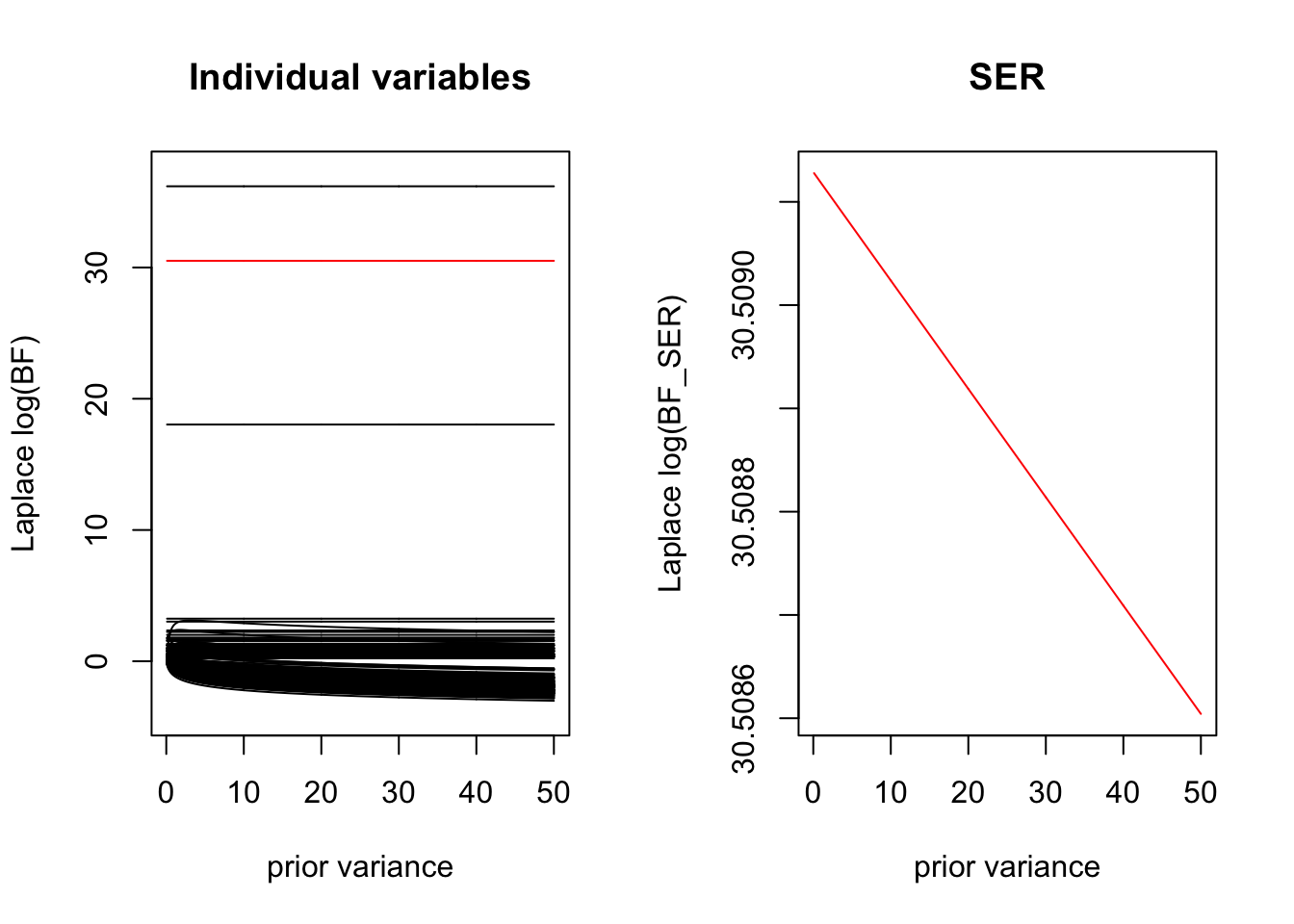
• When the estimated prior variance is \(0\) the Laplace approximation of the BF reduced to the LR, so the variables are just ranked by their LR.
• We estimate a very large prior variance of the third effect, but the CS is very diffuse. The 3rd effect includes all of the other completely enriched gene sets.

Code

knitr::knit_exit()

Code

fit <- logisticsusie::fit_glm_ser(X, y, estimate_prior_variance = T)

Code

# GIBSS fit
serfun <- purrr::partial(logisticsusie::uvbser, max_iter=2)

ser1 <- logisticsusie::uvbser(X, y1, max_iter = 20)

o <-( X %*% (ser1$mu * ser1$alpha))[,1]
ser2 <- logisticsusie::uvbser(X, y1, o = o,  max_iter = 20)

tic()
fit2 <- logisticsusie::ibss_from_ser(X, y1, L=5, maxit=2, ser_function = serfun)
toc()

Code

causal_idx <- which(colnames(X) %in% enriched_gs)
print(causal_idx)
fit$cs

Code

#' wrapper for VEB.boost to fit logistic susie
#' and tidy up output to be consistent with other susie-type outputs
fit_logistic_susie_veb_boost = function(X, y, L=10, ...){
  veb.fit = VEB.Boost::veb_boost_stumps(
    X, y, family = 'binomial',
    include_stumps=FALSE,
    max_log_prior_var=35,
    scale_X = 'NA',
    growMode = 'NA',
    changeToConstant=F,
    k=L, ...
  )
  
  alpha <- t(do.call(cbind, lapply(veb.fit$leaves, function(x) x$learner$currentFit$alpha)))
  mu <- t(do.call(cbind, lapply(veb.fit$leaves, function(x) x$learner$currentFit$mu)))
  mu2 <- t(do.call(cbind, lapply(veb.fit$leaves, function(x) x$learner$currentFit$sigma2_post)))
  mu2 <- mu2 + mu^2
  prior_variance <- purrr::map_dbl(veb.fit$leaves, function(x) x$learner$currentFit$V)
  elbo <- veb.fit$ELBO_progress[[2]]
  res <- list(alpha=alpha, mu=mu, mu2=mu2, elbo=elbo, veb.fit=veb.fit, prior_variance=prior_variance)
  class(res) <- 'susie'
  
  colnames(res$alpha) <- colnames(X)
  colnames(res$mu) <- colnames(X)
  res$pip <- susieR::susie_get_pip(res)
  names(res$pip) <- colnames(X)
  res$sets <- susieR::susie_get_cs(res, X=X)
  return(res)
}

tic()
vebfit <- fit_logistic_susie_veb_boost(X, y1, L=10)
toc()

Code

# JJ approximation-- VEB boost
tic()
veb_ser <- fit_logistic_susie_veb_boost(X, y1, L=1)
logisticsusie::compute_cs(veb_ser$alpha[1,])
toc()

# JJ approximation other implementation
tic()
jj_ser <- logisticsusie::binser(X, y1, estimate_prior_variance = F, prior_variance=veb_ser$prior_variance)
logisticsusie::compute_cs(jj_ser$alpha)
toc()

# veb and my implementation agree 
par(mfrow = c(1, 2))
plot(veb_ser$mu, jj_ser$mu); abline(0, 1, col='red')
plot(log(veb_ser$alpha), log(jj_ser$alpha)); abline(0, 1, col='red')

# SER fit with Laplace
serfit <- logisticsusie::generalized_ibss(X, y1, L=1, estimate_prior_variance = F, maxit=1)

plot(veb_ser$mu, serfit$mu); abline(0, 1, col='red')

# JJ approximation other implementation
tic()
jj_ser2 <- logisticsusie::binser(X, y1, estimate_prior_variance = F, prior_variance=serfit$prior_variance)
logisticsusie::compute_cs(jj_ser2$alpha)
toc()

# There is a difference between the GIBSS implementation and VB
par(mfrow = c(1, 2))
plot(serfit$mu, jj_ser2$mu); abline(0, 1, col='red')
plot(log(serfit$alpha), log(jj_ser2$alpha)); abline(0, 1, col='red')

# the ones that don't agree are completely separated-- the MLE does not exist.
# these may also inflate the estimated prior variance the VB approach?
# are are we underestimating the prior variance in the Laplace approximation?
weird <- (abs(serfit$mu[1,]) < 0.001) * (abs(jj_ser2$mu) > 0.001)
max((Matrix::t(X[,weird]) %*% y1)[,1])


# repeat with augmented data
Xaug <- rbind(X, matrix(rep(c(1, 1, 0, 0), ncol(X)), nrow=4))
y1aug <- c(y1, c(1, 0, 1, 0))

# JJ approximation-- VEB boost
tic()
veb_ser_aug <- fit_logistic_susie_veb_boost(Xaug, y1aug, L=1)
logisticsusie::compute_cs(veb_ser_aug$alpha[1,])
toc()

# JJ approximation other implementation
tic()
jj_ser_aug <- logisticsusie::binser(Xaug, y1aug, estimate_prior_variance = F, prior_variance=veb_ser$prior_variance)
logisticsusie::compute_cs(jj_ser_aug$alpha)
toc()

# veb and my implementation agree 
par(mfrow = c(1, 2))
plot(veb_ser_aug$mu, jj_ser_aug$mu); abline(0, 1, col='red')
plot(log(veb_ser_aug$alpha), log(jj_ser_aug$alpha)); abline(0, 1, col='red')

# SER fit with Laplace
serfit_aug <- logisticsusie::generalized_ibss(Xaug, y1aug, L=1, estimate_prior_variance = F, maxit=1)

# JJ approximation other implementation
tic()
jj_ser2_aug <- logisticsusie::binser(Xaug, y1aug, estimate_prior_variance = F, prior_variance=serfit$prior_variance)
logisticsusie::compute_cs(jj_ser2_aug$alpha)
toc()

# There is a difference between the GIBSS implementation and VB
par(mfrow = c(1, 2))
plot(serfit_aug$mu, jj_ser2_aug$mu); abline(0, 1, col='red')
plot(log(serfit_aug$alpha), log(jj_ser2_aug$alpha)); abline(0, 1, col='red')

Code

pi1 = 0.001
n <- 400
x <- rbinom(n, 1, pi1)
y <- rbinom(n, 1, pmin(rep(1, n), 0.1 + x))


fit <- fastglm::fastglm(x = as.matrix(cbind(rep(1, n), x)), y=y, family='binomial')


fit <- fastglm::fastglm(x = as.matrix(x, ncol=1) , y=y, family='binomial', intercept=T)


p1 <- mean(y[x==0])
p2 <- mean(y)

# compute lr directly
#a <- sum(dbinom(y, size=1, prob=1/(1 + exp(-predict(fit))), log=T)) - sum(dbinom(y, size=1, prob=p2, log=T))

# again
b <- sum(dbinom(y[x==0], size=1, prob=p1, log=T)) - sum(dbinom(y, size=1, prob=p2, log=T))

# from deviance
lr <- -0.5 * (fit$deviance - fit$null.deviance)

c(lr, b)

o <- rnorm(n)
fit <- glm(y ~ x + offset(o), family='binomial')
fit$null.deviance / 2

fit0 <- glm(y ~ 1 + offset(o), family='binomial')
fit0$deviance / 2

Quadrature

Code

fit_quad_ser2 <- function(X, y, o=NULL, prior_variance=1, ...){
  uvbser <- logisticsusie::fit_uvb_ser(X, y, o, prior_variance=prior_variance, ...)
  quadser <- logisticsusie::fit_quad_ser(
    X, y, o, prior_variance = prior_variance, glm_ser=uvbser, n=64, ...)
  return(quadser)
}

#gibssquad <- with(sim, logisticsusie::generalized_ibss_quad(X, y, L=5, n=32, estimate_prior_variance=F, maxit=10))

uvbser <- with(sim, logisticsusie::fit_uvb_ser(X, y, prior_variance=1.))
quad2 <- with(sim, fit_quad_ser2(X, y, prior_variance=1.))
plot(quad2$lbf, uvbser$lbf); abline(0, 1, col='red')

New section

No data augmentation, just explore the behvior of the different approximations

c1 simulation

Code

library(tictoc)
sim <- make_c1_sim()

loading gene set from msigdbr: C1

Code

# estimate prior variance with UVB
f <- function(prior_variance){
  with(sim, fit_uvb_ser(X, y, prior_variance=prior_variance, estimate_prior_variance=F))$lbf_model
}
#prior_variance <- optimize(f, c(1e-10, 100), maximum = T)$maximum
prior_variance = 66.63581

tic()
uvbser <- with(sim, logisticsusie::fit_uvb_ser(X, y, prior_variance=prior_variance))
toc()

4.345 sec elapsed

Code

# estimate prior variance with Laplace MLE
glmser <- with(sim, logisticsusie::fit_glm_ser(X, y, prior_variance=1, estimate_prior_variance=T))
abfser <- with(sim, logisticsusie::fit_glm_ser(X, y, prior_variance=1, estimate_prior_variance=T, laplace = F))

glue::glue('UVB estimated prior variance = {uvbser$prior_variance}\n Laplace estimated prior variance = {glmser$prior_variance}\n Wakefield estimated prior variance = {abfser$prior_variance}')

UVB estimated prior variance = 66.63581
Laplace estimated prior variance = 0
Wakefield estimated prior variance = 0

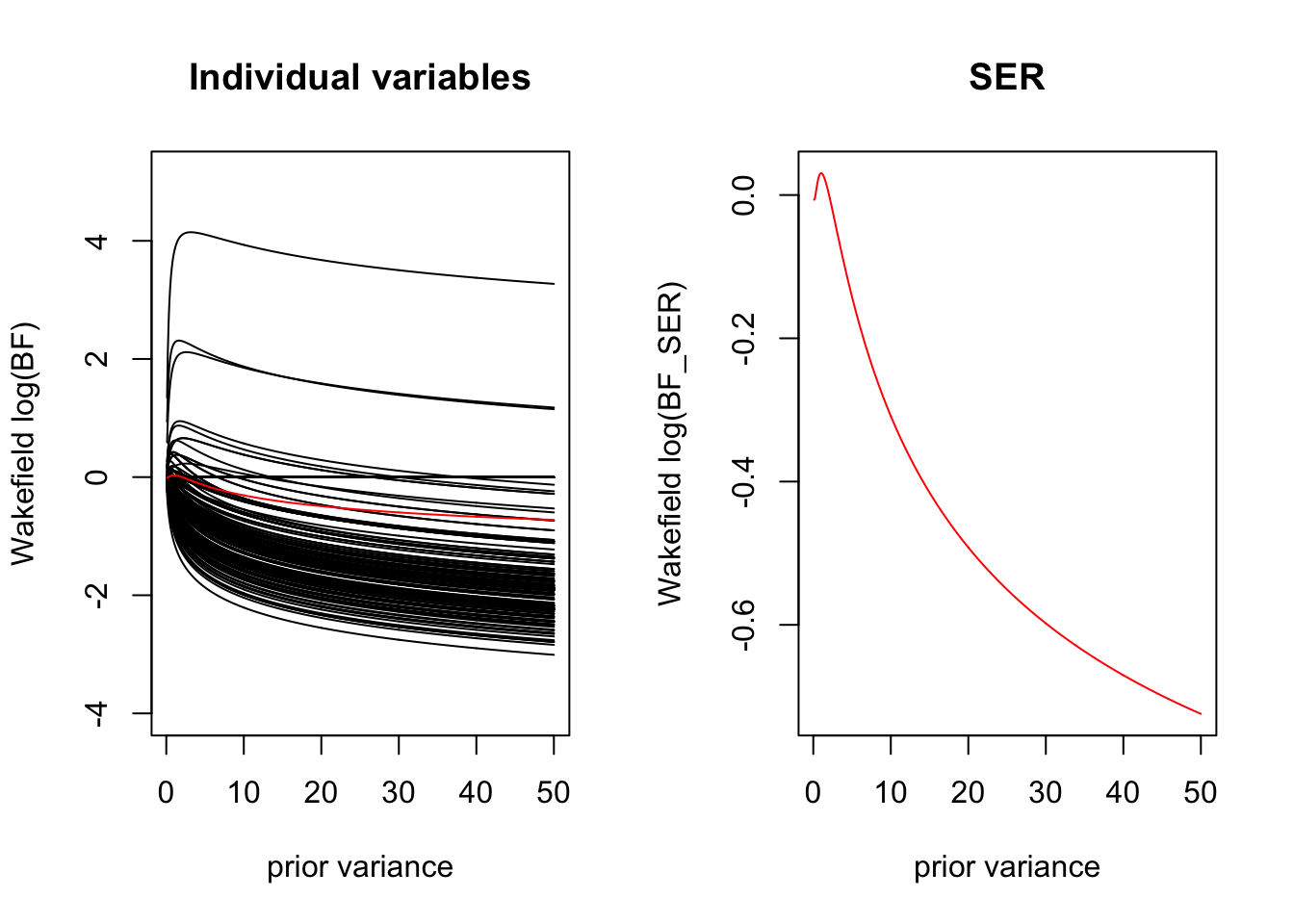
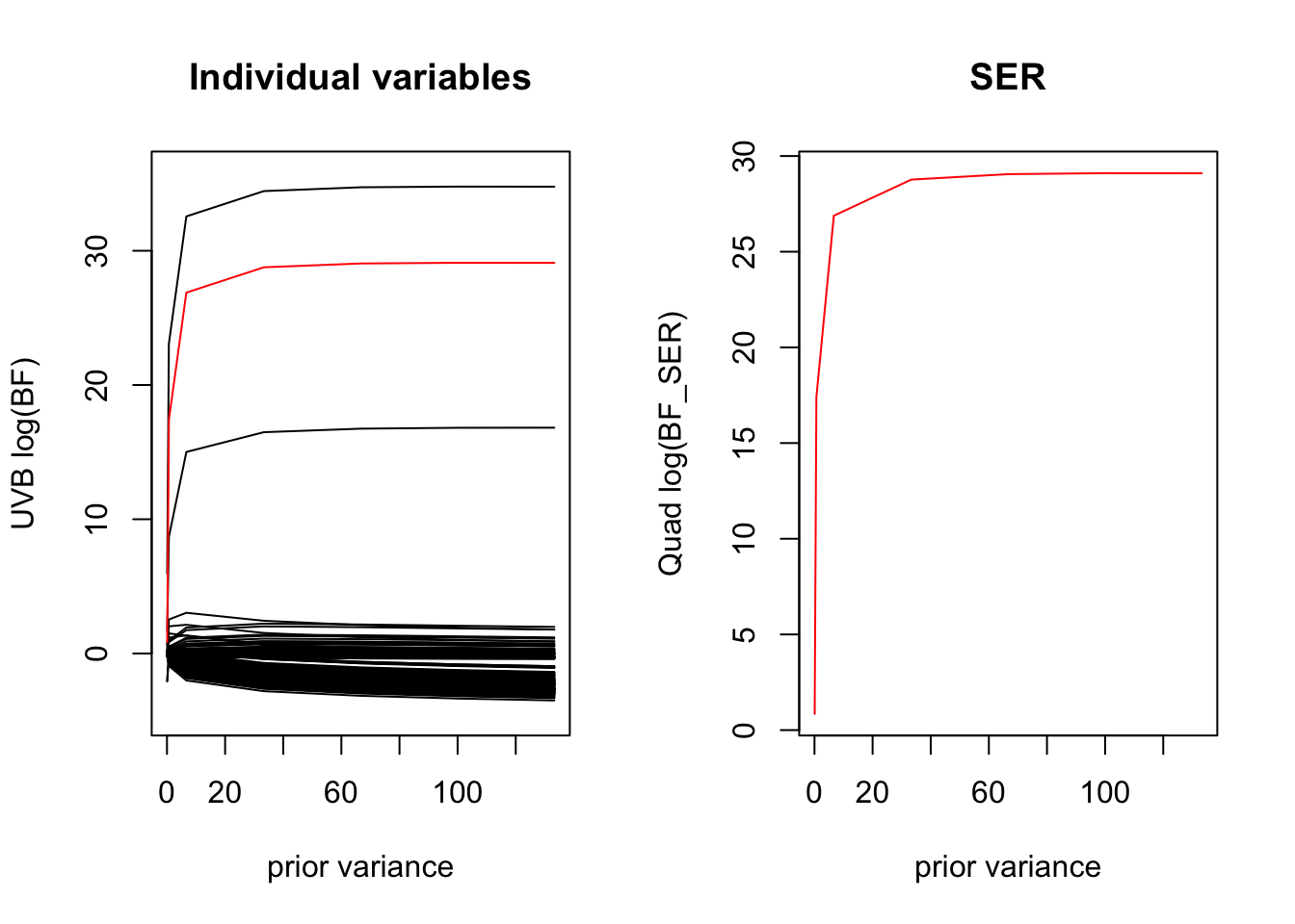
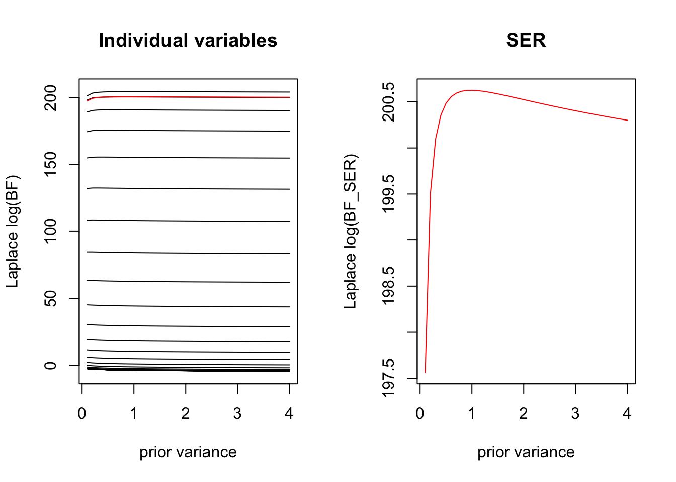
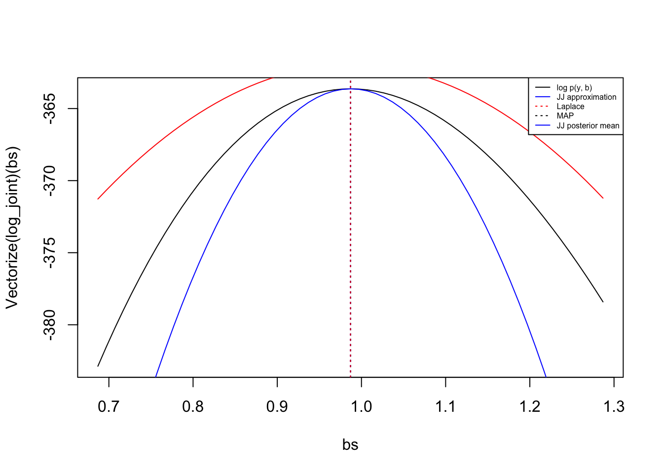
Here we plot how the BF varies as a function for the prior variance for each variable separately, and how this contributes to the overall BF for the SER. We see that for the variables that are completely enriched \(x=1 \implies y=1\) the Laplace BF is invariant to the choice of prior variance. Because there are many uninformative covariates, we are penalized for large settings of the prior variance.

Laplace

Code

# LAPLACE
f2 <- function(var0){with(glmser, logisticsusie:::compute_log_labf(betahat, shat2, lr, var0))}
sigma2_grid <- seq(0.1, 50, by=0.1)
laplace_log_bfs <- do.call('cbind', purrr::map(sigma2_grid, f2))

f3 <- function(var0){with(glmser, logisticsusie:::compute_log_labf_ser(betahat, shat2, lr, var0, pi = 1/length(betahat)))}
laplace_log_bf_sers <- purrr::map_dbl(sigma2_grid, f3)

# here we plot the in the laplace approximait
par(mfrow=c(1,2))
plot(sigma2_grid, laplace_log_bfs[1,], ylim = c(-1, 1) + range(laplace_log_bfs), type = 'l',  ylab = 'Laplace log(BF)', xlab = 'prior variance', main='Individual variables')
for(i in 2:nrow(laplace_log_bfs)){
  lines(sigma2_grid, laplace_log_bfs[i,], ylim = c(-1, 1) + range(laplace_log_bfs), type = 'l')
}
lines(sigma2_grid, laplace_log_bf_sers, col='red')
plot(sigma2_grid, laplace_log_bf_sers, col='red', type='l', ylab = 'Laplace log(BF_SER)', xlab = 'prior variance', main='SER')

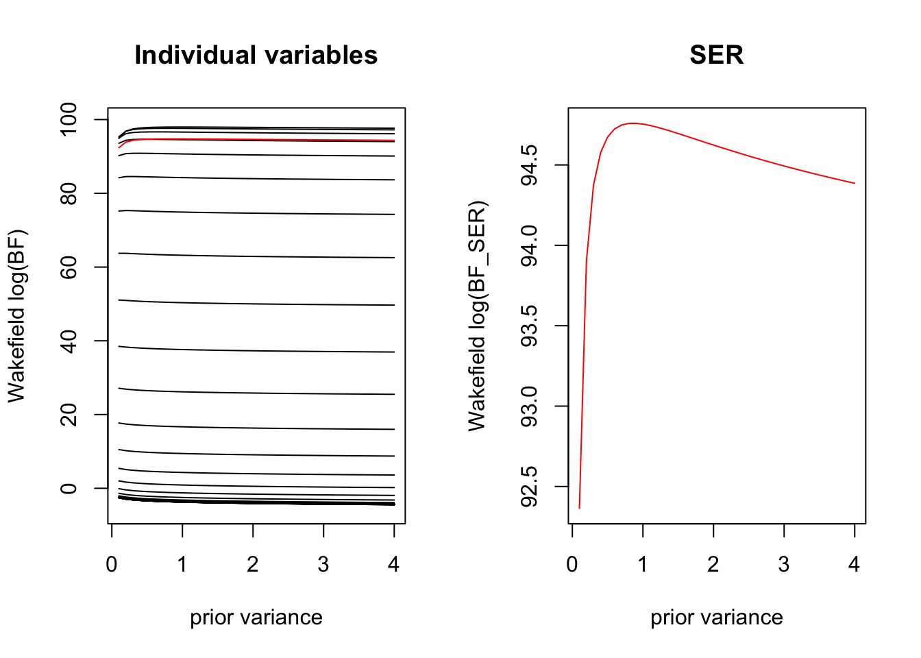
Wakefield

Code

# ABF
f4 <- function(var0){with(glmser, logisticsusie:::compute_log_abf(betahat, shat2, var0))}
sigma2_grid <- seq(0.1, 50, by=0.1)
log_abfs <- do.call('cbind', purrr::map(sigma2_grid, f4))

f5 <- function(var0){with(glmser, logisticsusie:::compute_log_abf_ser(betahat, shat2, var0, pi = 1/length(betahat)))}
log_abf_ser <- purrr::map_dbl(sigma2_grid, f5)

# here we plot the in the laplace approximait
par(mfrow=c(1,2))
plot(sigma2_grid, laplace_log_bfs[1,], ylim = c(-1, 1) + range(log_abfs), type = 'l',  ylab = 'Wakefield log(BF)', xlab = 'prior variance', main='Individual variables')
for(i in 2:nrow(log_abfs)){
  lines(sigma2_grid, log_abfs[i,], ylim = c(-1, 1) + range(log_abfs), type = 'l')
}
lines(sigma2_grid, log_abf_ser, col='red')
plot(sigma2_grid, log_abf_ser, col='red', type='l', ylab = 'Wakefield log(BF_SER)', xlab = 'prior variance', main='SER')

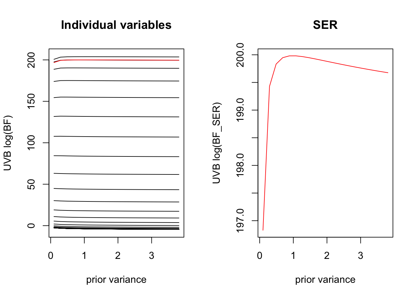
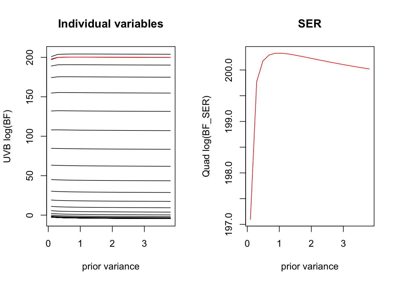
UVB

Code

sigma2_grid2 <- prior_variance * c(0.001, 0.01, 0.1, 0.5, 1.0, 1.5, 2.0) #0.1, 0.2,0.5, 1.0, 1.5, 2.0)
uvbsers <- purrr::map(sigma2_grid2, ~logisticsusie::fit_uvb_ser(sim$X, sim$y, prior_variance=.x))
log_bfs <- do.call('cbind', purrr::map(uvbsers, ~.x$lbf))
log_bf_ser <- do.call('cbind', purrr::map(uvbsers, ~.x$lbf_model))
# here we plot the in the laplace approximait
par(mfrow=c(1,2))
plot(sigma2_grid2, log_bfs[1,], ylim = c(-1, 1) + range(log_bfs), type = 'l',  ylab = 'UVB log(BF)', xlab = 'prior variance', main='Individual variables')
for(i in 2:nrow(log_bfs)){
  lines(sigma2_grid2, log_bfs[i,], ylim = c(-1, 1) + range(log_bfs), type = 'l')
}
lines(sigma2_grid2, log_bf_ser, col='red')
plot(sigma2_grid2, log_bf_ser, col='red', type='l', ylab = 'UVB log(BF_SER)', xlab = 'prior variance', main='SER')

Quadrature

Code

f6 <- function(prior_variance){
  ser <- uvbser
  ser$prior_variance <- prior_variance
  return(logisticsusie::fit_quad_ser(sim$X, sim$y, prior_variance=prior_variance, glm_ser=ser, n=32))
}
quadsers <- purrr::map(sigma2_grid2, f6)

logsumexp <- function(x){
  m <- max(x)
  return(m + log(sum(exp(x - m))))
}

log_bfs <- do.call('cbind', purrr::map(quadsers, ~.x$lbf))
log_bf_ser <- purrr::map_dbl(1:ncol(log_bfs), ~logsumexp(log_bfs[,.x] - log(nrow(log_bfs))))
#log_bf_ser <- do.call('cbind', purrr::map(quadsers, ~.x$lbf_model))

par(mfrow=c(1,2))
plot(sigma2_grid2, log_bfs[1,], ylim = c(-1, 1) + range(log_bfs), type = 'l',  ylab = 'UVB log(BF)', xlab = 'prior variance', main='Individual variables')
for(i in 2:nrow(log_bfs)){
  lines(sigma2_grid2, log_bfs[i,], ylim = c(-1, 1) + range(log_bfs), type = 'l')
}
lines(sigma2_grid2, log_bf_ser, col='red')
plot(sigma2_grid2, log_bf_ser, col='red', type='l', ylab = 'Quad log(BF_SER)', xlab = 'prior variance', main='SER')

Code

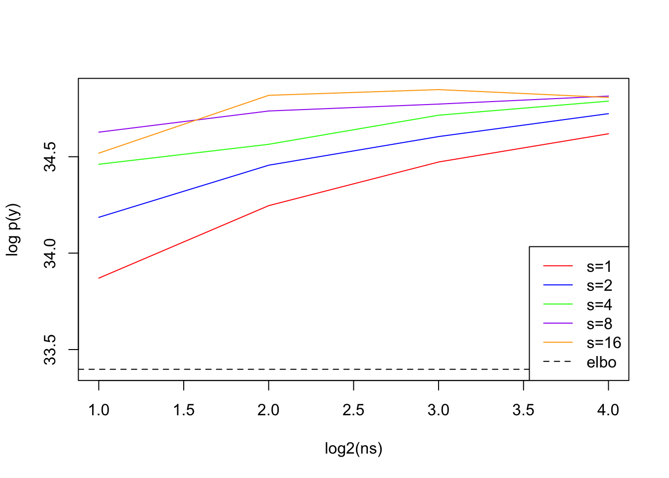
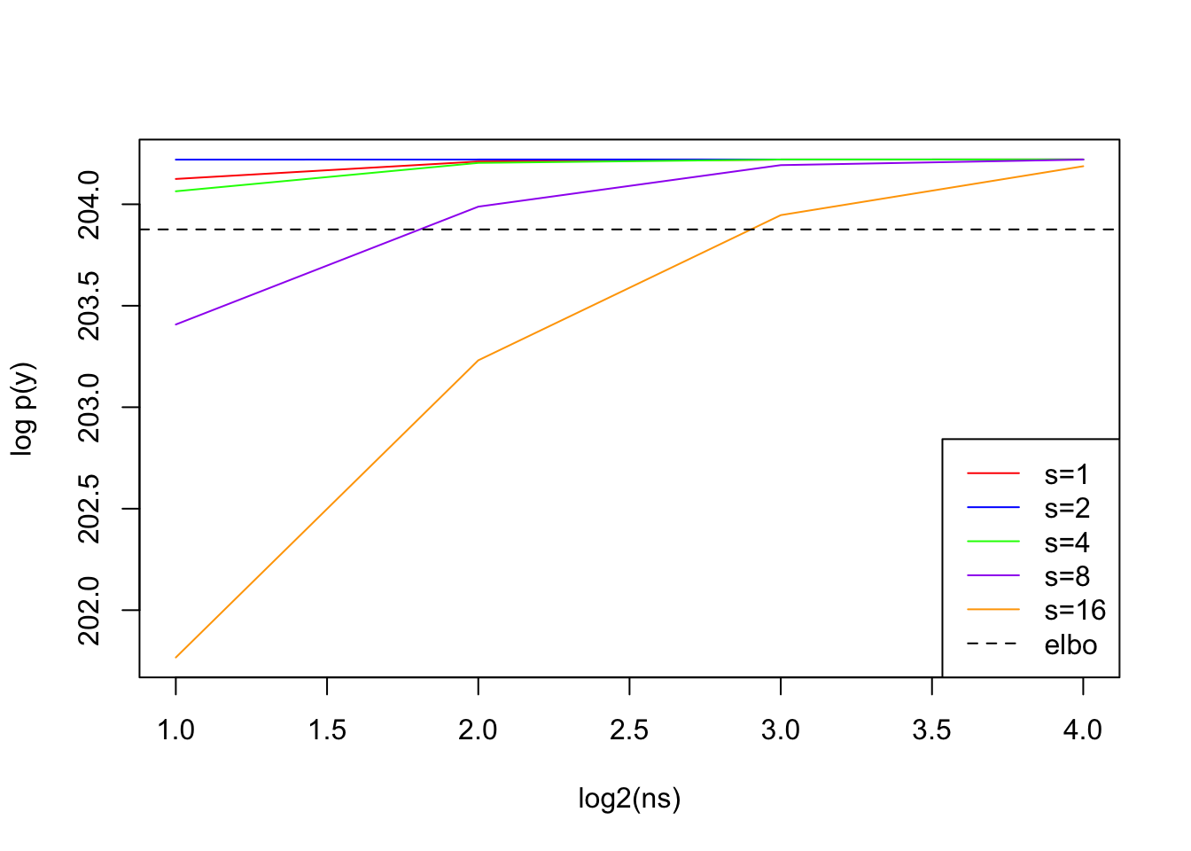
# QUADRATURE
# lets look at how Gauss-Hermite quadrature performs at a range of values (0, 1, 10, 66.39, 120)
x <- sim$X[,66]
y <- sim$y
jj_fit <- logisticsusie::fit_univariate_vb(x, y, tau0 = 1/prior_variance)
elbo <- tail(jj_fit$elbos, 1)
b0 <- jj_fit$delta
mu <- jj_fit$mu
var <- 1/jj_fit$tau

#' do Gauss-Hermite quadrature for a range of # of quadrature points
#' centered on the posterior mean, s is a rescaling of the posterior variance
quad_scale_variance <- function(ns, s, mu, var){
  purrr::map_dbl(ns, ~logisticsusie:::compute_log_marginal(
    x, y, b0 = b0, mu = mu, var = s*var, prior_variance = prior_variance, n=.x, verbose = F))
}

ns <- c(2, 4, 8, 16)
# suggests we can improve quadrature performance by
s1 <- quad_scale_variance(ns, 1, mu, var)
s2 <- quad_scale_variance(ns, 2, mu, var)
s4 <- quad_scale_variance(ns, 4, mu, var)
s8 <- quad_scale_variance(ns, 8, mu, var)
s16 <- quad_scale_variance(ns, 16, mu, var)

ll0 <- sum(dbinom(y, 1, mean(y), log=T))
ylim <- range(c(elbo - ll0, s1 - ll0, s2 - ll0, s4 - ll0, s8 - ll0, s16 - ll0))

plot(log2(ns), s1 - ll0, type='l', col='red', ylim=ylim, ylab = 'log p(y)')
lines(log2(ns), s2 - ll0, col='blue')
lines(log2(ns), s4 - ll0, col='green')
lines(log2(ns), s8 - ll0, col='purple')
lines(log2(ns), s16 - ll0, col='orange')
abline(h = elbo - ll0, lty=2) # plot elbo
abline(h = f3(prior_variance))
abline(h = f5(prior_variance))

legend(x ="bottomright",
       legend=c("s=1", "s=2", "s=4", "s=8", "s=16", 'elbo'),
       col = c("red","blue", "green", "purple", "orange","black"),
       lty = c(1, 1, 1, 1, 1, 2), cex=1.0)

Code

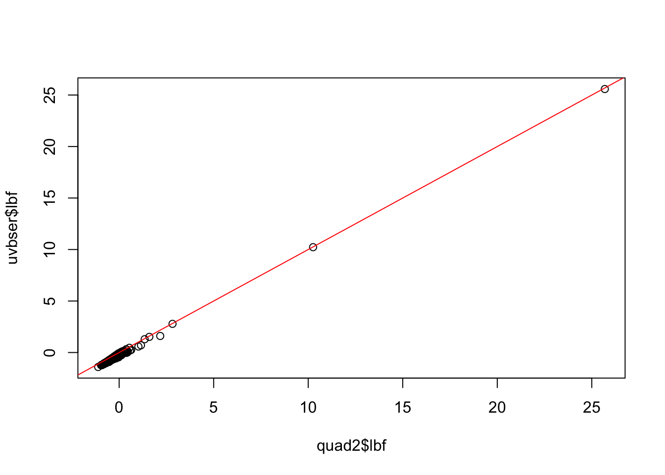
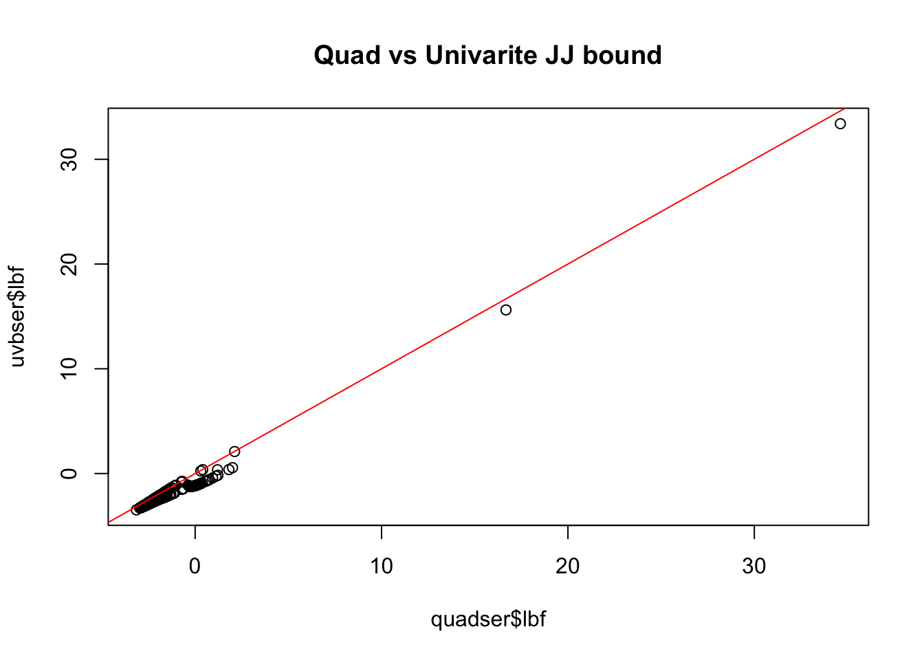
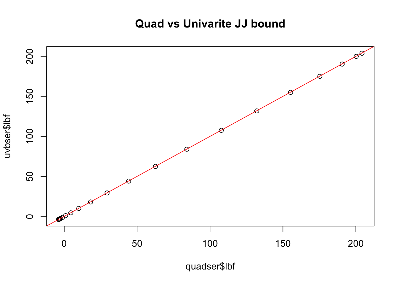
par(mfrow = c(1, 1))
sigmoid <- function(x){1 / (1 + exp(-x))}

quadser <- with(sim, logisticsusie::fit_quad_ser(X, y, prior_variance=prior_variance, glm_ser=uvbser, n=16))
plot(quadser$lbf, uvbser$lbf, main='Quad vs Univarite JJ bound'); abline(0, 1, col='red')

I also wanted to plot the Laplace approximation here but the MLE is too large and the approximate MAP estimate is too small to show up meaningfully on the plot

Code

log_joint <- function(b){
  psi <- b0 + x * b
  return(sum(y * psi - log(1 + exp(psi))) + dnorm(b, 0, sqrt(prior_variance), log=T))
}

xi <- jj_fit$xi
vb_bound <- function(b){
  psi <- b0 + x * b
  xs <- 2 * (y - 0.5) * psi
  lambda_xi <- (0.5 - sigmoid(xi)) / (2 * xi)
  bound <- sum(log(sigmoid(xi)) + 0.5 * (xs - xi) + lambda_xi *(xs^2 - xi^2)) + dnorm(b, 0, sqrt(prior_variance), log=T)
  return(bound)
}

glmser2 <- with(sim, logisticsusie::fit_glm_ser(X, y, prior_variance=prior_variance, estimate_prior_variance=F))
lap_log_joint <- function(b){
  mu <- glmser$mu[66]
  var <- glmser$var[66]
}

bs <- seq(mu-1, mu+0.5, by=0.01)

mu_opt <- optimize(log_joint, c(-10, 10), maximum = T)$maximum
plot(bs, Vectorize(log_joint)(bs), type='l')
abline(v = mu_opt, lty=3)

lines(bs, Vectorize(vb_bound)(bs), type='l', col='blue')
abline(v = mu, lty=3, col='blue')
legend(
  x = 'topright',
  legend = c('log p(y, b)', 'JJ approximation', 'MAP', 'JJ posterior mean'),
  col = c('black', 'blue'),
  lty = c(1, 1, 3, 3),
  cex=0.5
)

easy simulation

Code

library(tictoc)
sim <- logisticsusie::sim_ser()

# estimate prior variance with UVB
f <- function(prior_variance){
  with(sim, logisticsusie::fit_uvb_ser(X, y, prior_variance=prior_variance))$lbf_model
}
prior_variance <- optimize(f, c(1e-10, 100), maximum = T)$maximum

tic()
uvbser <- with(sim, logisticsusie::fit_uvb_ser(X, y, prior_variance=prior_variance))
toc()

0.073 sec elapsed

Code

# estimate prior variance with Laplace MLE
glmser <- with(sim, logisticsusie::fit_glm_ser(X, y, prior_variance=1, estimate_prior_variance=T))
abfser <- with(sim, logisticsusie::fit_glm_ser(X, y, prior_variance=1, estimate_prior_variance=T, laplace = F))

glue::glue('UVB estimated prior variance = {uvbser$prior_variance}\n Laplace estimated prior variance = {glmser$prior_variance}\n Wakefield estimated prior variance = {abfser$prior_variance}')

UVB estimated prior variance = 0.977334459751195
Laplace estimated prior variance = 0.978616418869904
Wakefield estimated prior variance = 0.978616418869904

Laplace

Code

# LAPLACE
f2 <- function(var0){with(glmser, logisticsusie:::compute_log_labf(betahat, shat2, lr, var0))}
sigma2_grid <- seq(0.1, 4, by=0.1)
laplace_log_bfs <- do.call('cbind', purrr::map(sigma2_grid, f2))

f3 <- function(var0){with(glmser, logisticsusie:::compute_log_labf_ser(betahat, shat2, lr, var0, pi = 1/length(betahat)))}
laplace_log_bf_sers <- purrr::map_dbl(sigma2_grid, f3)

# here we plot the in the laplace approximait
par(mfrow=c(1,2))
plot(sigma2_grid, laplace_log_bfs[1,], ylim = c(-1, 1) + range(laplace_log_bfs), type = 'l',  ylab = 'Laplace log(BF)', xlab = 'prior variance', main='Individual variables')
for(i in 2:nrow(laplace_log_bfs)){
  lines(sigma2_grid, laplace_log_bfs[i,], ylim = c(-1, 1) + range(laplace_log_bfs), type = 'l')
}
lines(sigma2_grid, laplace_log_bf_sers, col='red')
plot(sigma2_grid, laplace_log_bf_sers, col='red', type='l', ylab = 'Laplace log(BF_SER)', xlab = 'prior variance', main='SER')

Wakefield

Code

# ABF
f4 <- function(var0){with(glmser, logisticsusie:::compute_log_abf(betahat, shat2, var0))}
sigma2_grid <- seq(0.1, 4, by=0.1)
log_abfs <- do.call('cbind', purrr::map(sigma2_grid, f4))

f5 <- function(var0){with(glmser, logisticsusie:::compute_log_abf_ser(betahat, shat2, var0, pi = 1/length(betahat)))}
log_abf_ser <- purrr::map_dbl(sigma2_grid, f5)

# here we plot the in the laplace approximait
par(mfrow=c(1,2))
plot(sigma2_grid, log_abfs[1,], ylim = c(-1, 1) + range(log_abfs), type = 'l',  ylab = 'Wakefield log(BF)', xlab = 'prior variance', main='Individual variables')
for(i in 2:nrow(log_abfs)){
  lines(sigma2_grid, log_abfs[i,], ylim = c(-1, 1) + range(log_abfs), type = 'l')
}
lines(sigma2_grid, log_abf_ser, col='red')
plot(sigma2_grid, log_abf_ser, col='red', type='l', ylab = 'Wakefield log(BF_SER)', xlab = 'prior variance', main='SER')

UVB

Code

sigma2_grid2 <- prior_variance * seq(0.1, 4, by=0.2) #0.1, 0.2,0.5, 1.0, 1.5, 2.0)
uvbsers <- purrr::map(sigma2_grid2, ~logisticsusie::fit_uvb_ser(sim$X, sim$y, prior_variance=.x))
log_bfs <- do.call('cbind', purrr::map(uvbsers, ~.x$lbf))
log_bf_ser <- do.call('cbind', purrr::map(uvbsers, ~.x$lbf_model))
# here we plot the in the laplace approximait
par(mfrow=c(1,2))
plot(sigma2_grid2, log_bfs[1,], ylim = c(-1, 1) + range(log_bfs), type = 'l',  ylab = 'UVB log(BF)', xlab = 'prior variance', main='Individual variables')
for(i in 2:nrow(log_bfs)){
  lines(sigma2_grid2, log_bfs[i,], ylim = c(-1, 1) + range(log_bfs), type = 'l')
}
lines(sigma2_grid2, log_bf_ser, col='red')
plot(sigma2_grid2, log_bf_ser, col='red', type='l', ylab = 'UVB log(BF_SER)', xlab = 'prior variance', main='SER')

Quadrature

Code

f6 <- function(prior_variance){
  ser <- uvbser
  ser$prior_variance <- prior_variance
  return(logisticsusie::fit_quad_ser(sim$X, sim$y, prior_variance=prior_variance, glm_ser=ser, n=32))
}
quadsers <- purrr::map(sigma2_grid2, f6)

logsumexp <- function(x){
  m <- max(x)
  return(m + log(sum(exp(x - m))))
}

log_bfs <- do.call('cbind', purrr::map(quadsers, ~.x$lbf))
log_bf_ser <- purrr::map_dbl(1:ncol(log_bfs), ~logsumexp(log_bfs[,.x] - log(nrow(log_bfs))))
#log_bf_ser <- do.call('cbind', purrr::map(quadsers, ~.x$lbf_model))

par(mfrow=c(1,2))
plot(sigma2_grid2, log_bfs[1,], ylim = c(-1, 1) + range(log_bfs), type = 'l',  ylab = 'UVB log(BF)', xlab = 'prior variance', main='Individual variables')
for(i in 2:nrow(log_bfs)){
  lines(sigma2_grid2, log_bfs[i,], ylim = c(-1, 1) + range(log_bfs), type = 'l')
}
lines(sigma2_grid2, log_bf_ser, col='red')
plot(sigma2_grid2, log_bf_ser, col='red', type='l', ylab = 'Quad log(BF_SER)', xlab = 'prior variance', main='SER')

Code

# QUADRATURE
# lets look at how Gauss-Hermite quadrature performs at a range of values (0, 1, 10, 66.39, 120)
x <- sim$X[,1]
y <- sim$y
jj_fit <- logisticsusie::fit_univariate_vb(x, y, tau0 = 1/prior_variance)
elbo <- tail(jj_fit$elbos, 1)
b0 <- jj_fit$delta
mu <- jj_fit$mu
var <- 1/jj_fit$tau

#' do Gauss-Hermite quadrature for a range of # of quadrature points
#' centered on the posterior mean, s is a rescaling of the posterior variance
quad_scale_variance <- function(ns, s, mu, var){
  purrr::map_dbl(ns, ~logisticsusie:::compute_log_marginal(
    x, y, b0 = b0, mu = mu, var = s*var, prior_variance = prior_variance, n=.x, verbose = F))
}

ns <- c(2, 4, 8, 16)
# suggests we can improve quadrature performance by
s1 <- quad_scale_variance(ns, 1, mu, var)
s2 <- quad_scale_variance(ns, 2, mu, var)
s4 <- quad_scale_variance(ns, 4, mu, var)
s8 <- quad_scale_variance(ns, 8, mu, var)
s16 <- quad_scale_variance(ns, 16, mu, var)

ll0 <- sum(dbinom(y, 1, mean(y), log=T))
ylim <- range(c(elbo - ll0, s1 - ll0, s2 - ll0, s4 - ll0, s8 - ll0, s16 - ll0))

plot(log2(ns), s1 - ll0, type='l', col='red', ylim=ylim, ylab = 'log p(y)')
lines(log2(ns), s2 - ll0, col='blue')
lines(log2(ns), s4 - ll0, col='green')
lines(log2(ns), s8 - ll0, col='purple')
lines(log2(ns), s16 - ll0, col='orange')
abline(h = elbo - ll0, lty=2) # plot elbo
abline(h = f3(prior_variance))
abline(h = f5(prior_variance))

legend(x ="bottomright",
       legend=c("s=1", "s=2", "s=4", "s=8", "s=16", 'elbo'),
       col = c("red","blue", "green", "purple", "orange","black"),
       lty = c(1, 1, 1, 1, 1, 2), cex=1.0)

Code

par(mfrow = c(1, 1))
sigmoid <- function(x){1 / (1 + exp(-x))}

quadser <- with(sim, logisticsusie::fit_quad_ser(X, y, prior_variance=prior_variance, glm_ser=uvbser, n=16))
plot(quadser$lbf, uvbser$lbf, main='Quad vs Univarite JJ bound'); abline(0, 1, col='red')

Ah– something odd about the Laplace approximation plot…

Code

log_joint <- function(b){
  psi <- b0 + x * b
  return(sum(y * psi - log(1 + exp(psi))) + dnorm(b, 0, sqrt(prior_variance), log=T))
}

xi <- jj_fit$xi
vb_bound <- function(b){
  psi <- b0 + x * b
  xs <- 2 * (y - 0.5) * psi
  lambda_xi <- (0.5 - sigmoid(xi)) / (2 * xi)
  bound <- sum(log(sigmoid(xi)) + 
                 0.5 * (xs - xi) + lambda_xi *(xs^2 - xi^2)) + 
    dnorm(b, 0, sqrt(prior_variance), log=T)
  return(bound)
}

glmser2 <- with(glmser, logisticsusie:::asymptotic_ser(betahat, shat2, intercept, lr, laplace=T, prior_variance = prior_variance, prior_weights = 1/length(betahat)))
ll0 <- with(sim, sum(dbinom(y, 1, mean(y), log=T)))

lap_log_joint <- function(b){
  mu <- glmser2$mu[1]
  var <- glmser2$var[1]
  tau <- 1/glmser$shat2[1]
  tau0 <- 1/glmser$prior_variance
  ll <- glmser2$lr[1] + ll0
  return(ll - 0.5/var * (b - mu)^2 + dnorm(b, 0, sd=sqrt(prior_variance)))
}

bs <- seq(mu-0.3, mu+0.3, by=0.01)

mu_opt <- optimize(log_joint, c(-10, 10), maximum = T)$maximum
plot(bs, Vectorize(log_joint)(bs), type='l')
abline(v = mu_opt, lty=3)

lines(bs, Vectorize(vb_bound)(bs), type='l', col='blue')
abline(v = mu, lty=3, col='blue')

lines(bs, Vectorize(lap_log_joint)(bs), type='l', col='red')
abline(v = mu, lty=3, col='red')
legend(
  x = 'topright',
  legend = c('log p(y, b)', 'JJ approximation', 'Laplace', 'MAP', 'JJ posterior mean'),
  col = c('black', 'blue', 'red'),
  lty = c(1, 1, 3, 3),
  cex=0.5
)

what’s the point?

1. UVB SER seems reliable for estimating the prior variance, unlike Laplace or Wakefield
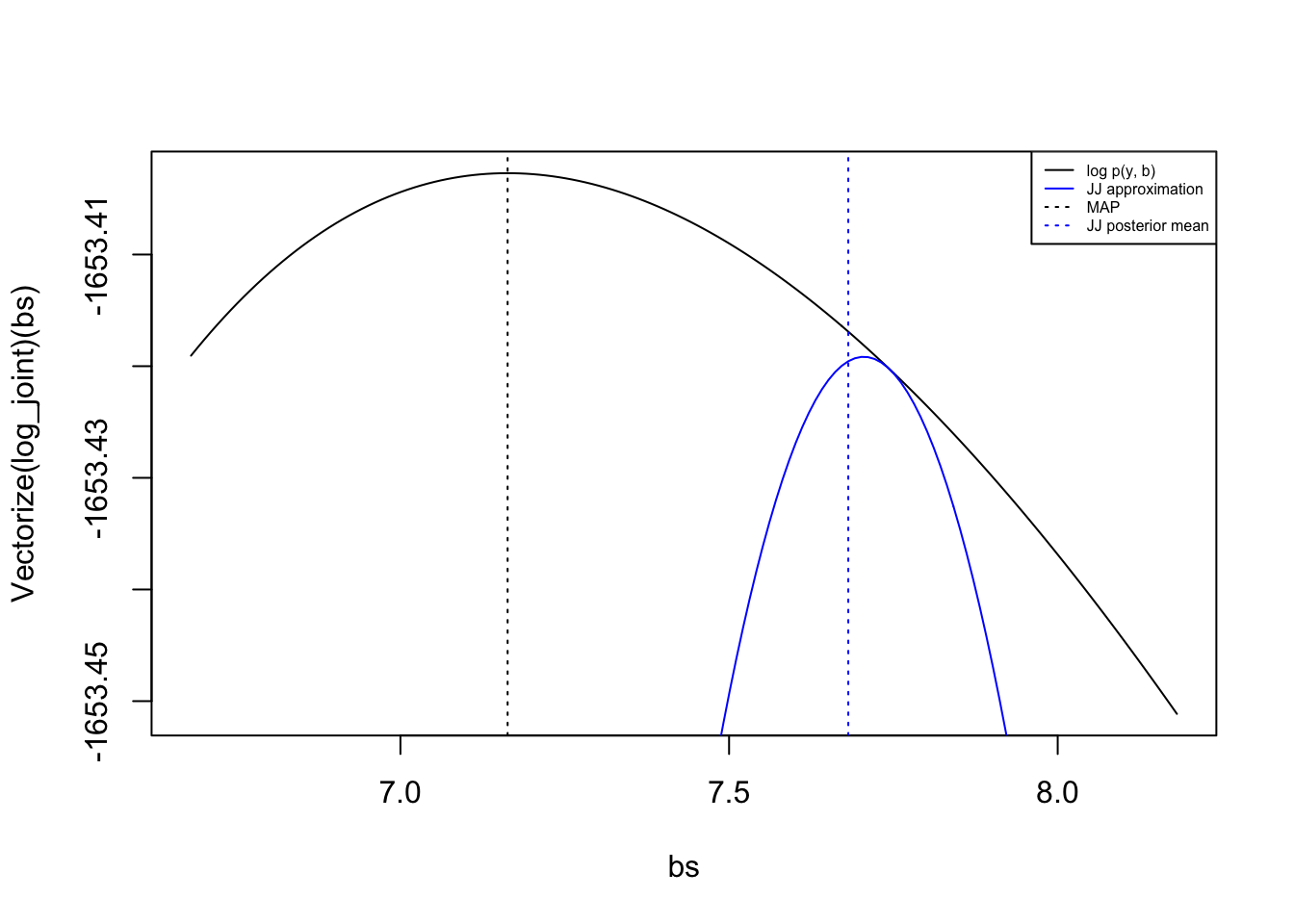
2. However, we can dramatically underestimate the posterior variance– which is a problem if we are determining the ‘width’ of the Gauss-Hermite quadrature. In well behaved situations 2 quadrature points is sufficient, but if we’ve underestimated the variance it takes many more points to get a good approximation.