Variational Objective
log joint:
\[\begin{align}
F(\beta_1, \dots, \beta_L) &= \log p(y | \sum_l(\psi_l)) + \sum_{l=1}^L\log p(\psi_l), \\
\psi_l &= X \beta_l, \\
\beta_l &\sim g_l
\end{align}\]
ELBO:
\[\begin{align}
\mathcal F(q_1, \dots, q_L) &= \mathbb E_q \left[ F(\beta_1, \dots \beta_L) \right] + \sum_l H(q_l) \\
q(\beta_1, \dots, \beta_L) &= \prod q_l(\beta_l)
\end{align}\]
Mode rather than mean?
\[\begin{align}
F(\beta_1, \dots, \beta_L) &= \log p(y | \sum_l(\psi_l)) + \sum_{l=1}^L\log p(\psi_l), \\
\end{align}\]
\[\begin{align}
\beta_l^* = \arg\max_{\beta_l} F(\beta_1, \dots, \beta_L)
\end{align}\]
Notes:
- Converges to a mode of the posterior.
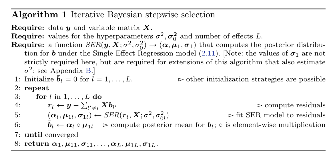
- Just iterative stepwise regression with fixed \(L\).
- Seems undesirable to include \(\beta_l\) for effects with weak evidence.
- Resembles CAVI when \(q(\gamma_l)\) is concentrated on highly correlated variables.
- Can still report SER posteriors for each effect \(l\).
A
\[\begin{align}
\mathcal F(q_1, \dots, q_L) = \mathbb E_q \left[ F(\beta_1, \dots \beta_L) \right] + \sum_l H(q_l)
\end{align}\]
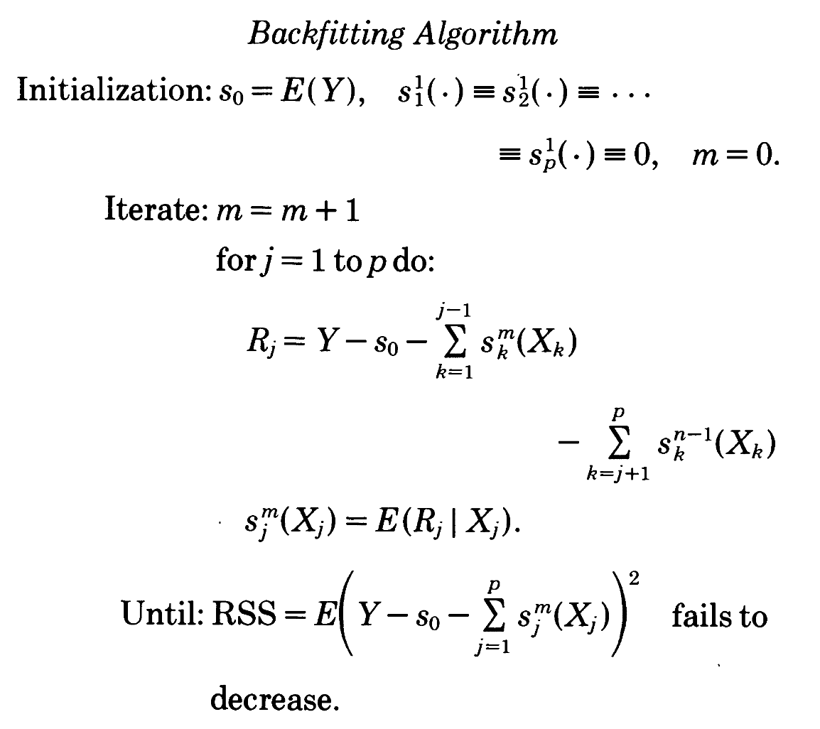
Coordinate ascent on \((\beta_l)\). For SuSiE, at each step fit an SER, but only return the posterior mode of the SER, rather than the mean. Essentially stepwise selection, but reports a posterior distribution for each effect. ## Backfitting
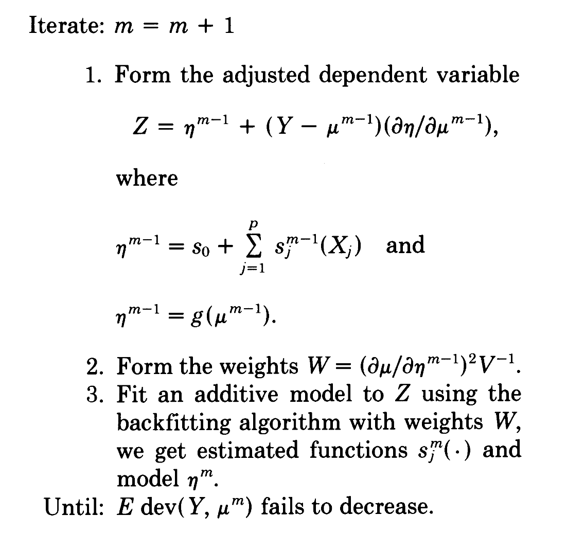
Maximize the expected log likelihood
\[
\begin{align}
\mathbb E[ l(\hat{\eta}(X), Y)] = \max_{\eta} \mathbb E[l(\eta(X), Y)]
\end{align}
\]
Overview
- Publication plan:
- Generalized SuSiE via IBSS, emphasis on fine-mapping for non-Gaussian models
- GSEA with logistic SuSiE
Fine-mapping under the multivariate Gaussian model
Most fine-mapping methods assume summary statistics from marginal association studies are normally distributed, with covariance determined by LD 1
\[\begin{align*}
\hat{ {\bf z} } \sim N({\bf z}, R)
\end{align*}\]
Statistical property of OLS– what if the marginal effects are coming from somewhere else?
What do we want to accomplish?
- Establish when there is a problem with fine-mapping with summary stats from non-Gaussian models
- (Hopefully) find that these situations are not uncommon
- (Hopefully) demonstrate that GIBSS offers improvement in these situations
- (Fallback) advise people to fine map with summary statistics from linear models
Three horse race
| Generalized IBSS |
“correct” model, hueristic algorithm |
No |
| Logistic + RSS |
ad-hoc, actually used (8,9) |
Yes |
| Linear + RSS |
mis-specified model, correct algorithm |
Yes |
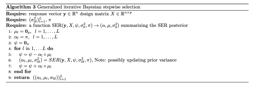
GIBSS overview
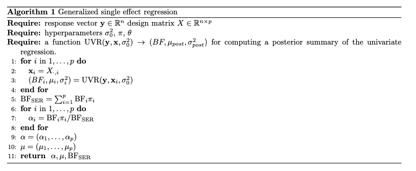
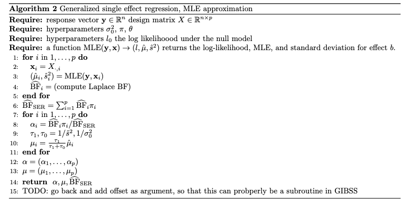
- Compute univariate effect estimates using regression of choice, must return MLE and stderr
- Compute/approximate BFs and posterior means: Laplace, quadrature, etc.
- Use predictions as fixed offsets when updating next effect
- Iterate until
convergence (we don’t know if it converges)
Potential problems
Logistic + RSS
- Covariate of marginal \(z\)-scores do not correspond with LD
- Under appreciated source of “LD Mismatch?”
- Follow-up: what is the correct covariance matrix?
- Inherits problems from using ABF– not the most accurate
Logistic GIBSS
- Marginal effect estimates are biased when there is a large genetic component
Correlation of marginal effects in logistic regression:
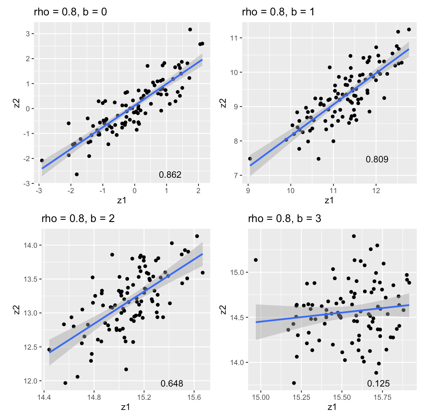
- Simulate \(\begin{bmatrix}x_1 \\ x_2 \end{bmatrix} \sim N(\begin{bmatrix}0 \\ 0 \end{bmatrix}, \begin{bmatrix}1 & \rho \\ \rho & 1 \end{bmatrix})\)
- Simulate \(y\) under a logistic model \(y \sim Bin(1, \sigma(\psi)), \; \psi := b_0 + b x_1\)
- \(cor(z_1, z_2) \neq \rho \implies\) LD matrix is the wrong covariance matrix
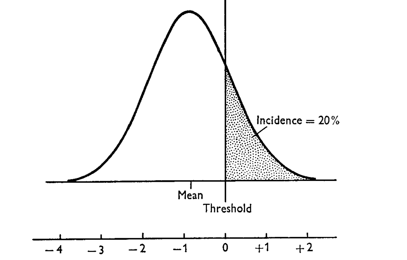
Correlation of marginal effects (cont)
An under-appreciated source of “LD mismatch”?
\(n = 500\), \(b_0 = -1\), \(b = 0, 1, 2, 3\) 1
![]()
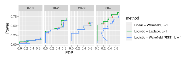
Laplace vs Wakefield (Review)
Figure 2: Wakefield’s ABF can be order of magnitude off when the \(z\)-score is large
Problems with Wakefield (Review)
!()[resources/abf_biased.png]
!()[resources/abf_eq.png]
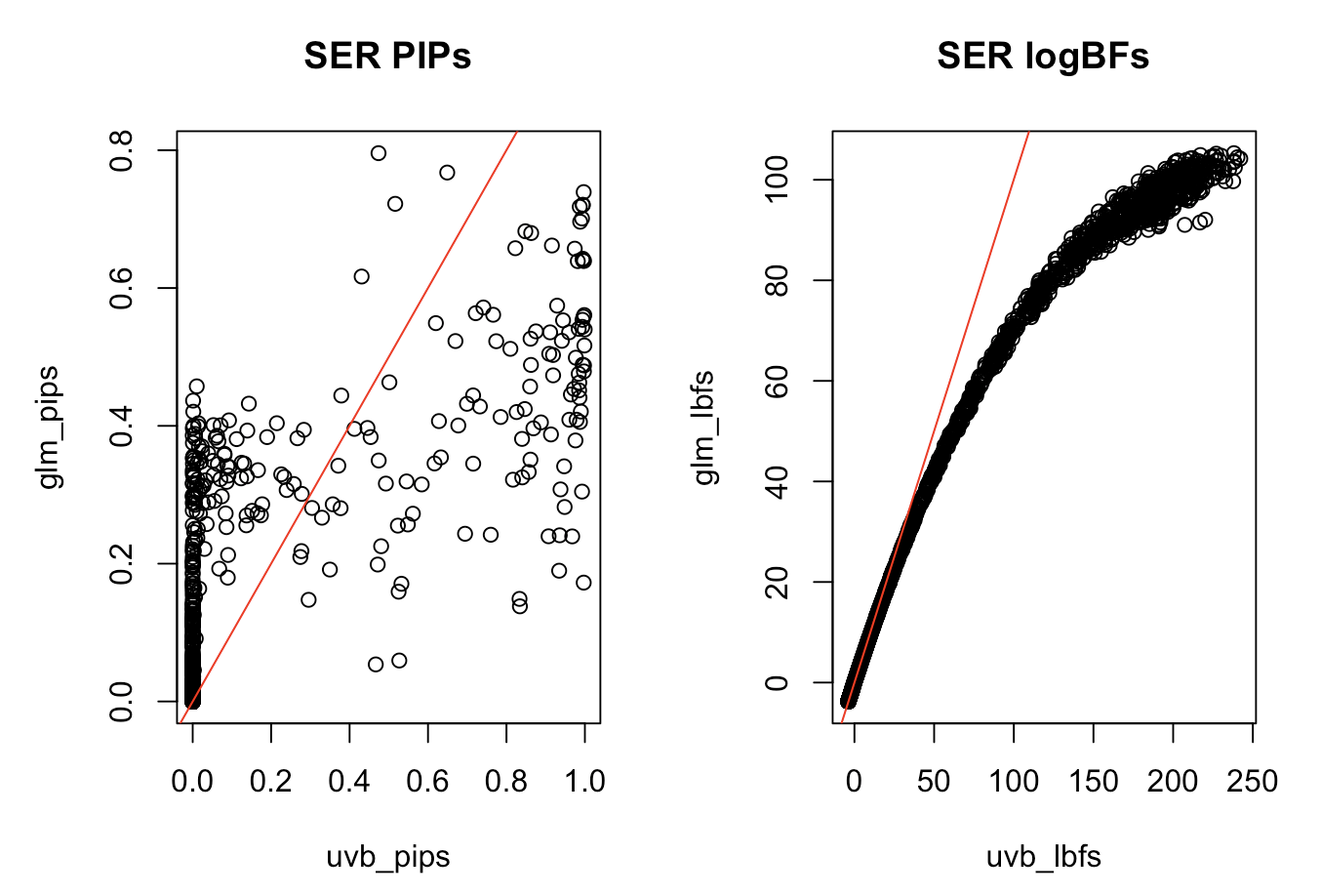
SuSiE-RSS and the Wakefield BF
- Recall that Wakefield’s ABF is not accurate when the \(z\)-score is large
- Applying SuSiE-RSS to summary statistics from some other model besides Gaussian linear model
How large do the \(z\)-scores need to be?
![]()
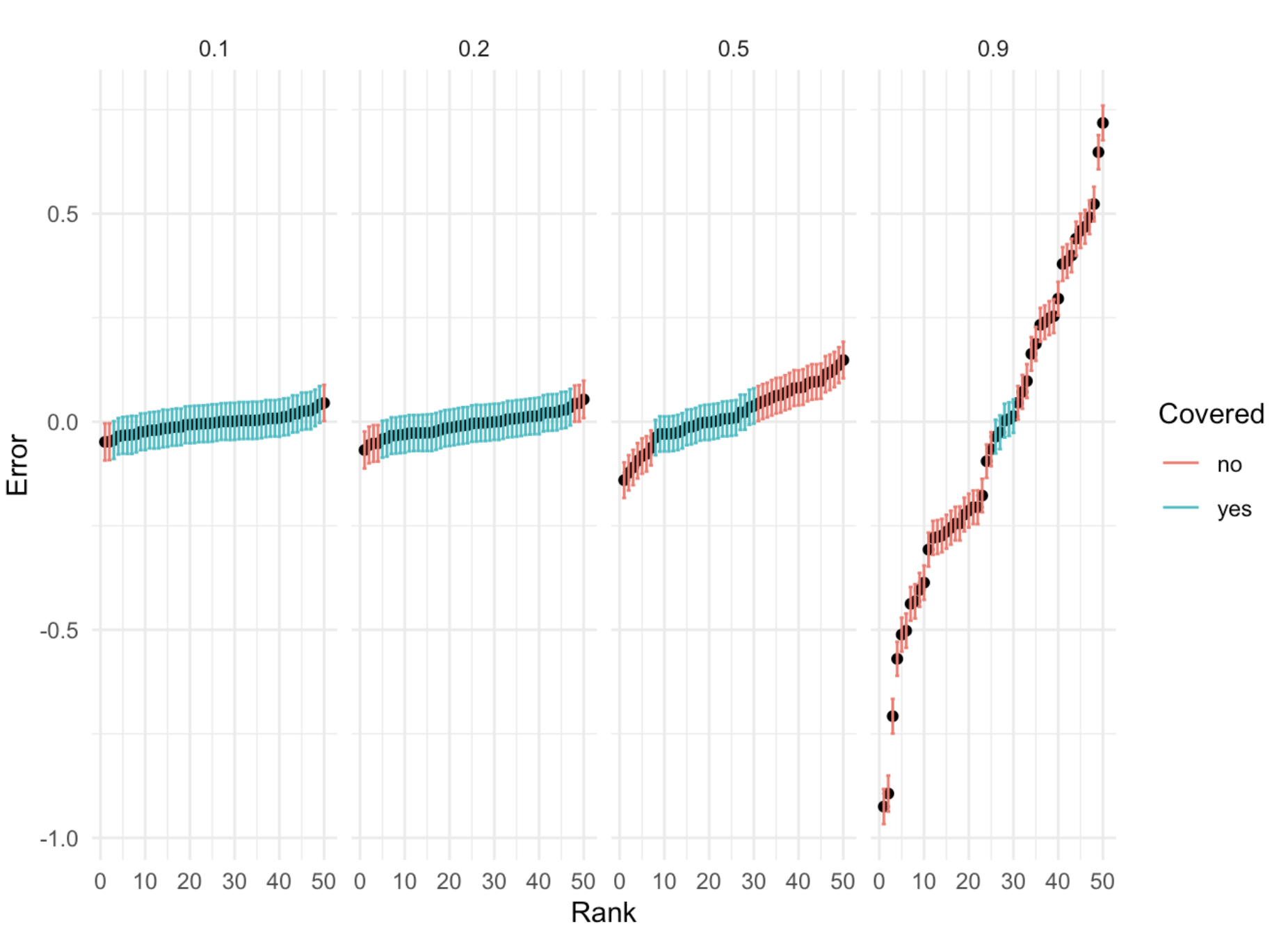
Biased effect estimates (and BFs)
Simulation: one causal variant in the locus that explains \(1\%\) of heritability of liability. \(h^2 = 0.1, 0.2, 0.5, 0.9\)
\[\begin{align*}
y \sim Bin(1, \sigma(\psi)) \\
\psi = b_0 + b x + \epsilon \\
\epsilon \sim N(0, \sigma^2)
\end{align*}\]
Biased effect estimates (and BFs)
![]()
Biased effect estimates (and BFs)
![]()
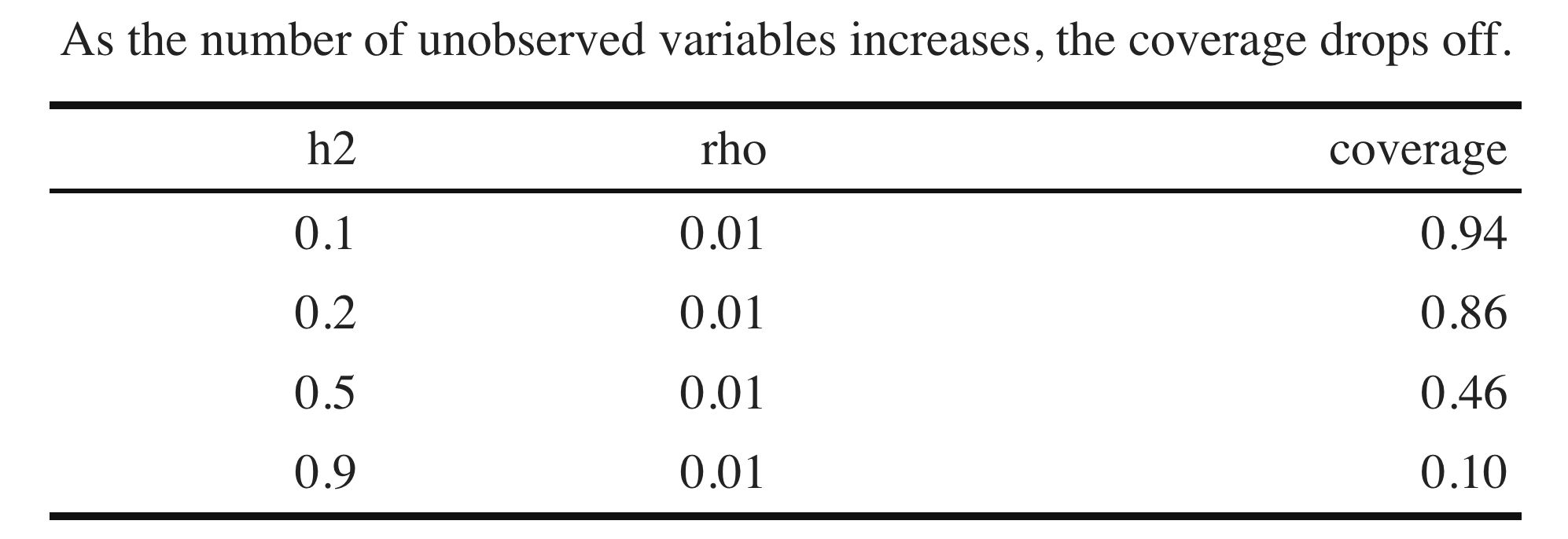
95% C.I. for different \(h^2\)
Biased effect estimates (and BFs)
- For phenotypes with substantial \(h^2\) of liability, restricting our attention to a single locus will lead to biased effect estimates
- Remark: linear model doesn’t struggle with this issue because in practice we estimate the residual variance (or set conservatively)
- Remark:basically a random intercept model, but this seems a little different than the usual motivation for mixed model approaches.
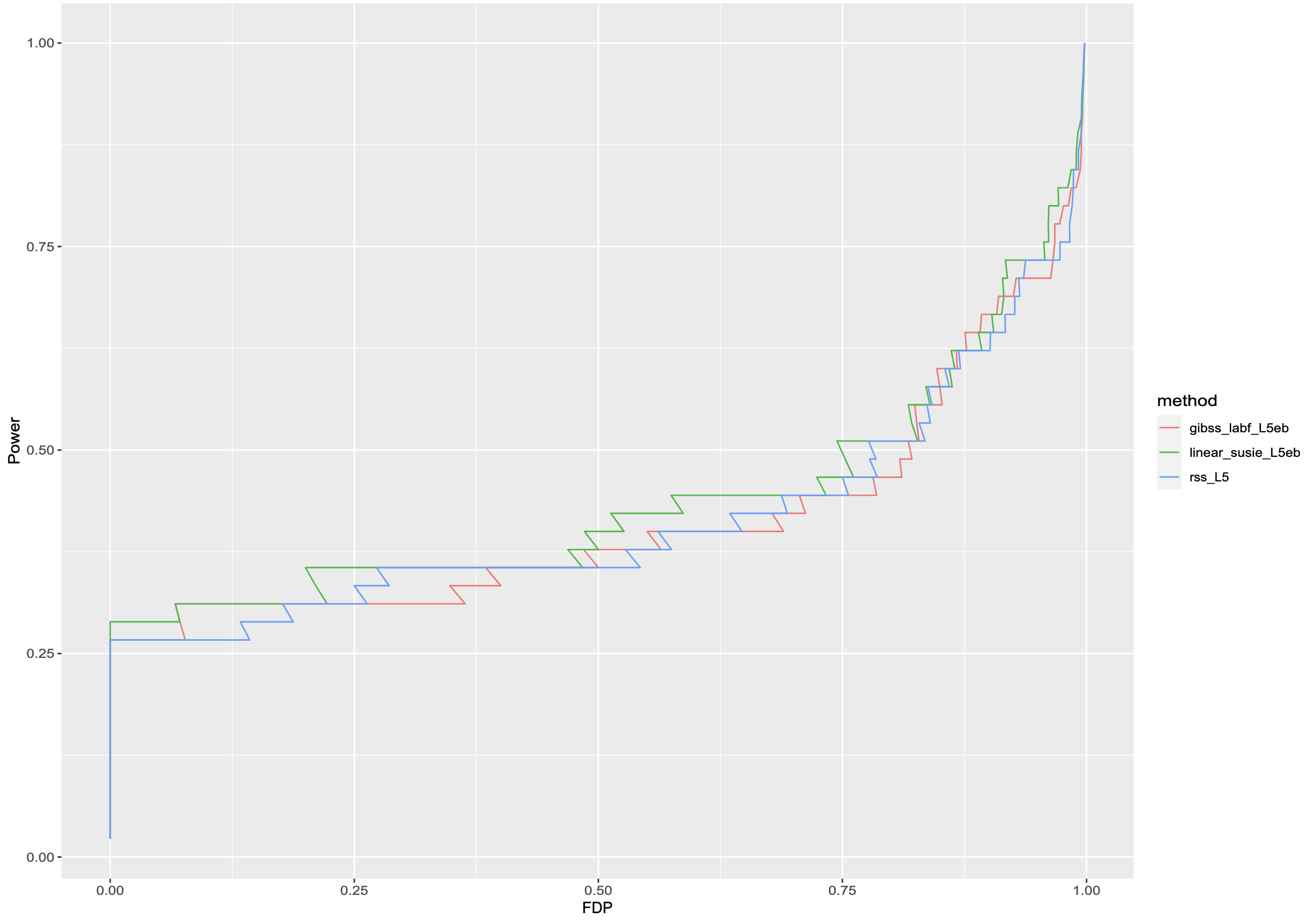
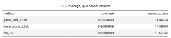
Real data analsis
- Q: if we reun SuSiE, GIBSS, Logistic + RSS on real case-control GWAS do we get qualitatively different results?
- Don’t know ground truth, hard to tell what is performing better
- Replication failure rate (RFR) among PIPs proposed in (10) may support claim that using GIBSS > Linear + RSS > Logistic + RSS
- Other ideas?
- Do you know of imbalanced case-control GWAS, survival GWAS, etc. GWAS on count based phenotypes, etc to test out?
Examples where SuSiE is applied to non-Gaussian linear summary stats
(8), Alzheimers meta analysis combining linear and logistic association studies (9) logistic-mixed model SAIGE + SuSiE
Dealing with intercept + covariates
A few options:
- Estimate in outer loop, treat as a fixed offset while estimating SERs
- Re-estimate covariate effects for each variable
- Found that reestimating intercept was helpful
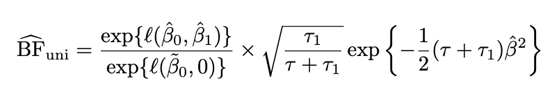
Univariate BF
![]()
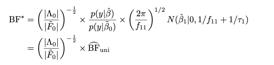
Limiting BF
Limiting BF
Idea put a normal prior on all covariates \(\begin{bmatrix} \alpha \\ \beta \end{bmatrix} \sim N(\begin{bmatrix} 0 \\ 0 \end{bmatrix}, \begin{bmatrix} I_{p-1} \tau_0^{-1} & 0 \\ 0 & \tau_1^{-1} \end{bmatrix}\) and compute Laplace approximation to the BF. Take \(\tau_0 \rightarrow 0+\).
![]()
Q: How variable is the scaling factor? Can we get away with just using the univariate BF?
Better quadrature rule
Gauss-Hermite quadrature
\[
I = \int f(x) e^{-x^2} dx \approx \sum_{i=1}^n w_i f(x_i)
\]
\((x_i)_{i=1}^n\) are the roots of the Hermite polynomial \(H_n(x)\), \(w_i = \frac{2^{n-1} n! \sqrt{\pi}}{n^2 H_{n-1}^2 (x_i)}\)
\[
I = \int f(x) dx = \int \left[\frac{f(x)}{q(x)} \right] q(x) dx, \;\; q(x) = N(x | \mu, \sigma^2)\; \text{s.t.}\; \frac{f}{q} \approx 1
\]
- Asymptotically correct
- Otherwise, integrating a function with little variation where the integrand has mass
- Upshot: very accurate integrals with e.g. \(n = 8, 16\).
(note: change of variable + scaling factor to apply the \(n\) point Hermite quadrature rule)