Gilad Lab WIP

Karl Tayeb

7/26/23

Polynomial SuSiE Updates

Last domino: constructing base approximation

Recall: if we find a good polynomial approximation to the log-likelihood for each observation we can cheaply approximate inference in the non-conjugate model
Previous strategy: Chebyshev interpolating polynomials can approximately minimize \(||f - \hat f||_{\infty}\) on a target interval.
Problem: interpolating polynomials are not guarunteed to have negative leading coefficient (a requirement for this approach)
What is a general strategy for computing legal polynomial approximations?

Generalized IBSS

Yet another approach to GLM-SuSiE

SuSiE: model

\[ \begin{aligned} y &\sim N(X\beta, \sigma^2_0) \\ \beta &= \sum_l b_l \gamma_l \\ b_l &\sim N(0, \sigma^2_0)\\ \gamma_l &\sim \text{Multinomial}(1, \pi) \end{aligned} \]

Variational inference

Inference as an optimization problem:

\[\begin{align} p(\beta | {\bf y}, X) = \arg \max_q F(q), \quad F(q) := \mathbb E_q \left[ \log p ({\bf y} | X, \beta) \right] - KL[q || p] \end{align}\]

\[\begin{align} F(q) &= \mathbb E_q \left[ \log p ({\bf y} | X, \beta) \right] - KL[q || p] \\ &= \mathbb E_q \left[ \log p ({\bf y}, \beta | X) \right] + H(q) \\ &= \left(\mathbb E_q \left[ \log p ({\bf y}, \beta | X) - Z \right] + H(q) \right) + Z \\ &= - KL[q || p_{post}] + Z \end{align}\]

We’ll write the variational objective for SER \(F_{SER}(q; {\bf y}, X, \sigma_0)\)

SuSiE: variational approximation

Restrict \(q\) to some family \(\mathcal Q\)

\[\begin{align} q^*(\beta) = \arg \max_{q \in \mathcal Q} F(q) \end{align}\]

SuSiE uses \(\mathcal Q = \{q : q(\beta) = \prod_l q_l(\beta_l)\}\)

\[ F_{SuSiE}(q; X, {\bf y}) = \mathbb E_{q} \left[ -\frac{1}{2\sigma^2}||{\bf y} - {\bf X} \beta_{-l} - X\beta_l||^2_2) \right] + KL[q || p_{SuSiE}] + C(\sigma) \]

SuSiE: coordinate ascent (IBSS)

Define the residual \({\bf r}_l = {\bf y} - X\beta_{-l}\)

\[ \begin{aligned} F_{SuSiE}(q_l; q_{-l}, X, {\bf y}) &= \mathbb E_{q_l} \left[ \mathbb E_{q_{-l}} \left[ -\frac{1}{2\sigma^2}||{\bf y} - {\bf X} \beta_{-l} - X\beta_l||^2_2) \right] \right] - KL[q || p] \\ &= \mathbb E_{q_l} \left[ \mathbb E_{q_{-l}} \left[ -\frac{1}{2\sigma^2}|| {\bf r}_l - X\beta_l||^2_2) \right] \right] - KL[q_l || p_l] + C_1 \\ &= \mathbb E_{q_l} \left[ \color{blue}{ -\frac{1}{2\sigma^2} \left(|| \mathbb E_{q_{-l}} {\bf r}_l- X\beta_l||^2_2 + \mathbb V ||r_l||^2_2 \right)} \right] - KL[q_l || p_l] + C_1\\ &= \mathbb E_{q_l} \left[ -\frac{1}{2\sigma^2} || \mathbb E_{q_{-l}} {\bf r}_l- X\beta_l||^2_2] \right] - KL[q_l || p_l] + C_2 \\ &= F_{SER}(q_l; X, \mathbb E_{q{-l}}{\bf r}_l) + C_2 \end{aligned} \]

Key: coordinate updates in \(\mathcal Q\) reduce to solving an SER

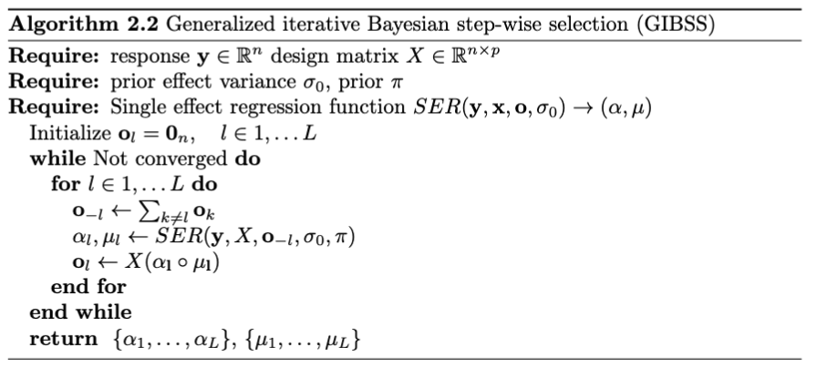
Generalized IBSS (GIBSS)

Heuristic approach for applying SuSiE to non-Gaussian models
Idea: apply IBSS, using expected predictions as fixed offsets

\[\begin{align} F_{SuSiE}(q) &= \mathbb E_q[\log p({\bf y} | X, \beta_l, \beta_{-l})] - \sum_l KL[q_l || p_l] \\ &= \mathbb E_{q_l}[ \mathbb E_{q_{-l}}[\log p({\bf y} | X, \beta_l, \beta_{-l})]] - \sum_l KL[q_l || p_l] + C_1 \\ &\color{purple}{\approx \mathbb E_{q_l}[\log p({\bf y} | X, \beta_l, \bar \beta_{-l})] - KL[q_l || p_l] + C_2} \\ &= F_{SER}(q_l; {\bf y}, X, \bar \beta_{-l}) + C_2 \end{align}\]

Why should this work?

\[ \begin{aligned} F_{SuSiE}(q) &= \mathbb E_q[\log p({\bf y} | X, \beta_l, \beta_{-l})] - \sum_l KL[q_l || p_l] \\ &\color{purple}{\approx \mathbb E_{q_l}[\log p({\bf y} | X, \beta_l, \bar \beta_{-l})] - KL[q_l || p_l] + C_2} \\ \end{aligned} \]

If \(\log p( {\bf y} | X, \beta)\) is quadratic in \(\beta\) (Gaussian) there \(\color{purple}\approx\) is \(=\)
Informally, approximation is good if \(\log p( {\bf y} | X, \beta)\) is well approximated by a quadratic function in \(\beta\).
Really we care about \(\psi = X\beta\)

Algorithm: Single effect regression

Require a function \(G\) which computes the BF and posterior mean of a Bayesian univariate regression

\[\begin{align} {\bf y} \sim 1 + {\bf x} + {\bf o} \\ b \sim N(0, \sigma^2) \end{align}\]

Advantage and limitations

Advantages

Seems to work well!
Highly modular: just need to implement the univariate regression

Disadvantages

Heuristic– not optimizing a clear objective function
Does not properly account for uncertainty in \(\beta_{-l}\), only uses posterior mean

Opportunities

Can we analyze the approximation error?
Can we make guarantees on GIBSS performance asymptotically?

Sources of error

GIBSS with exact SER

Treating random effects as fixed effects (only need to pass posterior means)

GIBSS with asymptotic approximation

Asymptotic approximation of posterior means (only need to compute MLE and std. errors)
Approximation of BFs

Algorithm: GIBSS

Simulations

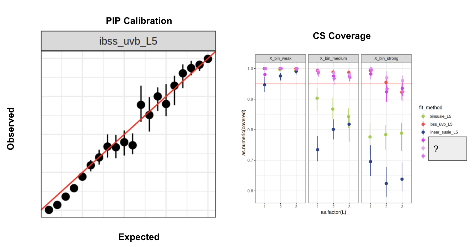
Simulations: logistic-GIBSS \(L=5\)

Much better performance compared to direct VB approach

Lasso simulation

Fit lasso to each gene list, simulate new gene lists from lasso fit (x20) - Gene sets: MSigDb Hallmark + C2 - ~7500 genes, ~4500 gene sets

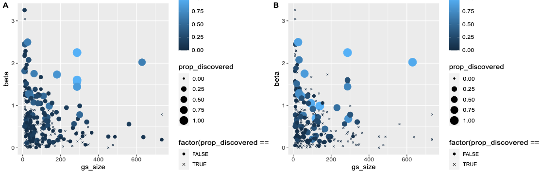
Lasso simulation CS summary

Some of the CSs are large (uninformative)

“Confident” discoveries 260/527 vs lasso 460 effects
SuSiE has good CS coverage ~94%
Lasso has high FP rate ~34%

# Causal x CS size	1	2	3	4	5	6	7	8	9	12
0	17	3	1	0	0	0	1	0	0	0
1	244	6	4	2	2	0	1	0	1	0
2	0	14	1	0	0	1	0	1	0	1
3	0	0	0	1	0	2	0	0	0	0
4	0	0	0	0	1	1	0	0	0	0

GIBSS for logistic regression

Goal: demonstrate improvement from using Laplace ABF over ABF in GIBSS for settings commonly found in case-control GWAS

Implication: Naive application of “summary stat” based finemapping methods not appropriate for e.g. logistic regression, GLMs, GLMMs.

Realistic simulation plan

UKBB genotype data

Simulate from UKBB imputed genotypes
Select 50k individual per UKBB, keep SNPs with MAF > 1% in sample

Simulation parameters

\[ \begin{aligned} y_i \sim Bernoulli(p_i) \\ \log \frac{p_i}{1 - p_i} = \beta_{0i} + \beta x_i\\ \beta_{0i} \sim N(b_0, \sigma^2_0) \\ \beta \sim N(0, \sigma^2) \end{aligned} \]

Random intercept models genetic contributions at un-linked loci, larger \(\sigma^2_0\) means focal SNP explains smaller fraction of \(h^2\)
\(\sigma^2\) should be selected to reflect un-normalized effect sizes in GWAS
Tune \(b_0\), \(\sigma^2_0\) to reflect case-control ratios and polygenecity of trait

This simulation

\[ \begin{aligned} y_i \sim Bernoulli(p_i) \\ \log \frac{p_i}{1 - p_i} = \beta_{0i} + \beta x_i\\ \beta_{0i} \sim N(b_0, \sigma^2_0) \\ \beta \sim N(0, \sigma^2) \end{aligned} \]

Random intercept models genetic contributions at un-linked loci, larger \(\sigma^2_0\) means focal SNP explains smaller fraction of \(h^2\)
\(\sigma^2\) should be selected to reflect un-normalized effect sizes in GWAS
Tune \(b_0\), \(\sigma^2_0\) to reflect case-control ratios and polygenecity of trait

\(\sigma^2_0 = 0\) (fixed intercept)
Select causal SNP to have MAF in \((0.2, 0.25)\)
Tuned \(b_0\) to give frequency of cases to approx. \(1 - 10\%\)
50 replicates on one region of chromosome 1.

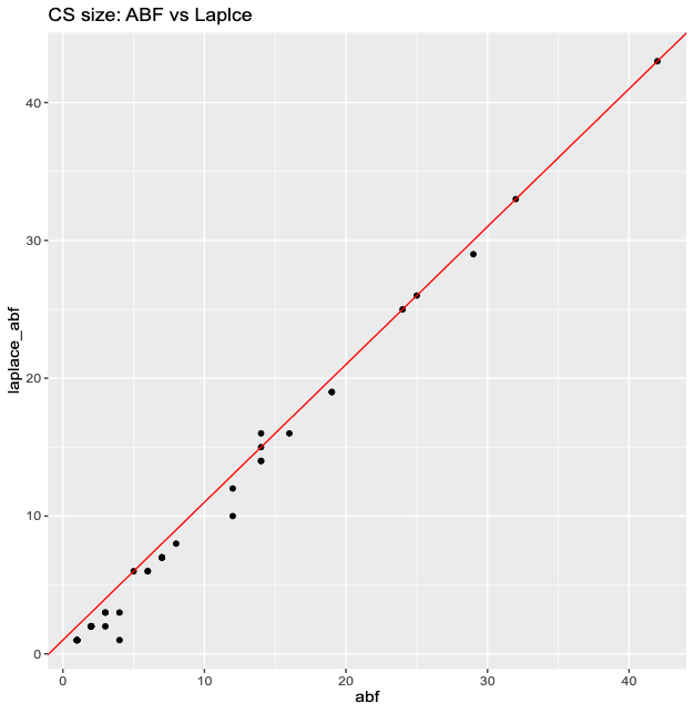
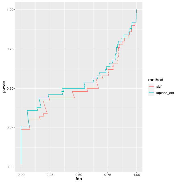
Logistic SuSiE ABF vs Laplace

95% CS coverage
Method	Coverage
abf	0.953
laplace_abf	0.977

{fig-align=“right”, height=10%}

GIBSS for survival analysis

Yunqi has been investigating specifically the application of SuSiE for survival analysis.

‘Non-standard’: optimization of partial likelihood to get MLE and standard error, censored data
Fits within the GIBSS framework!

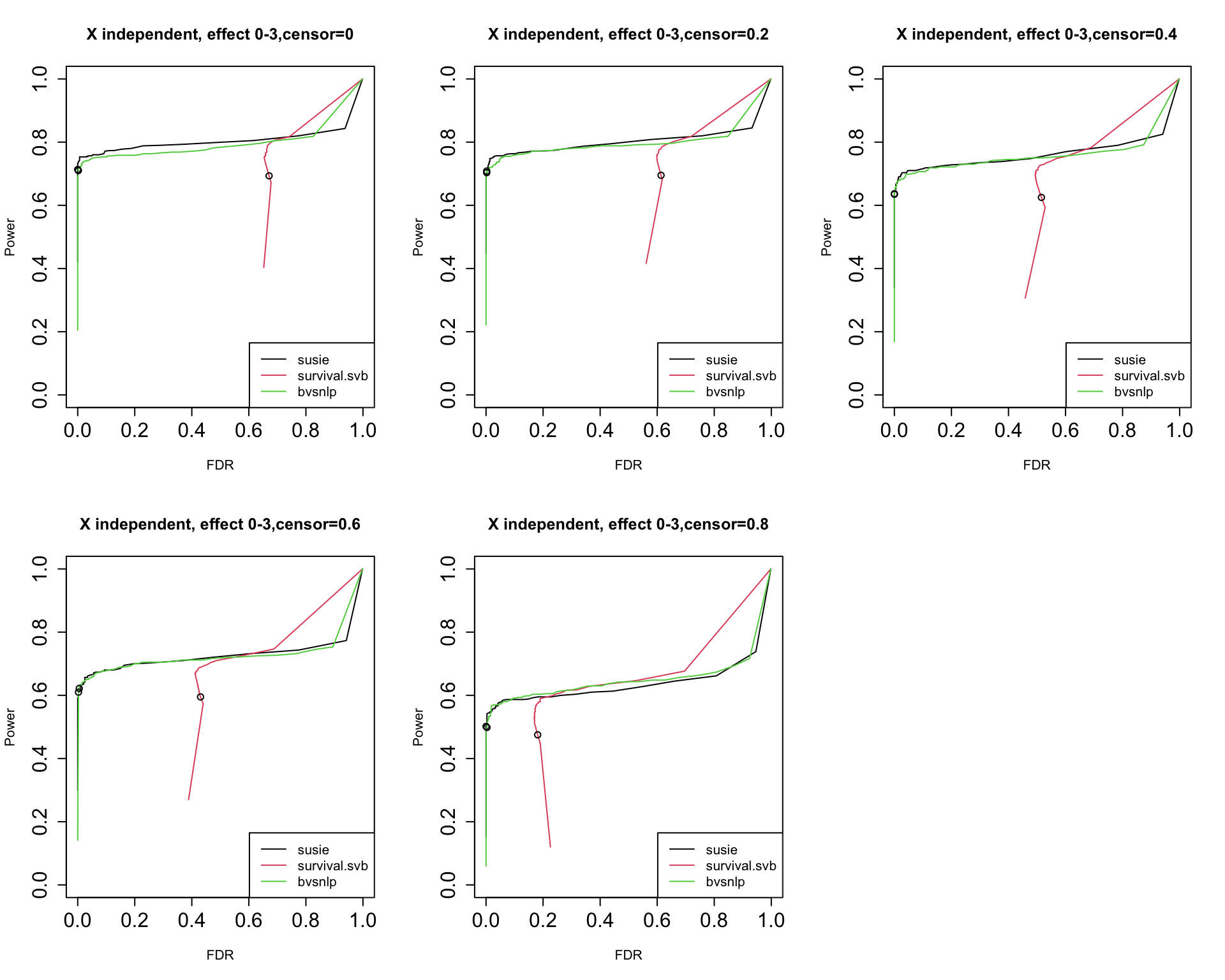
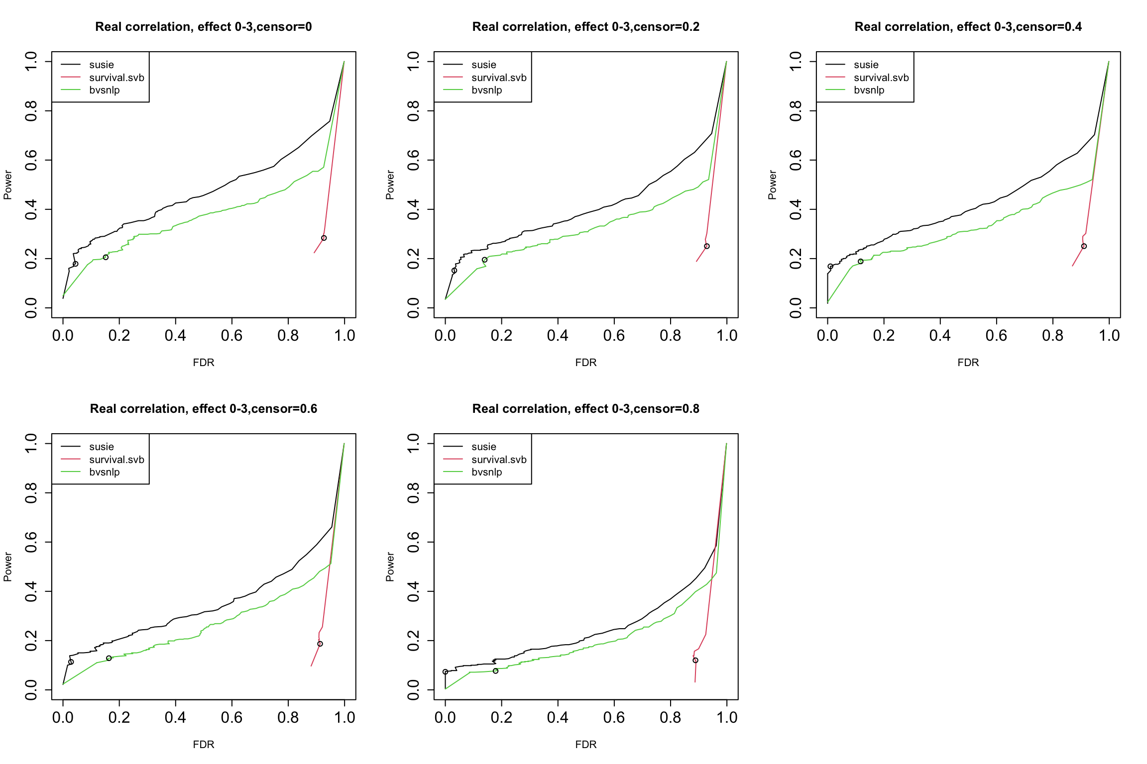
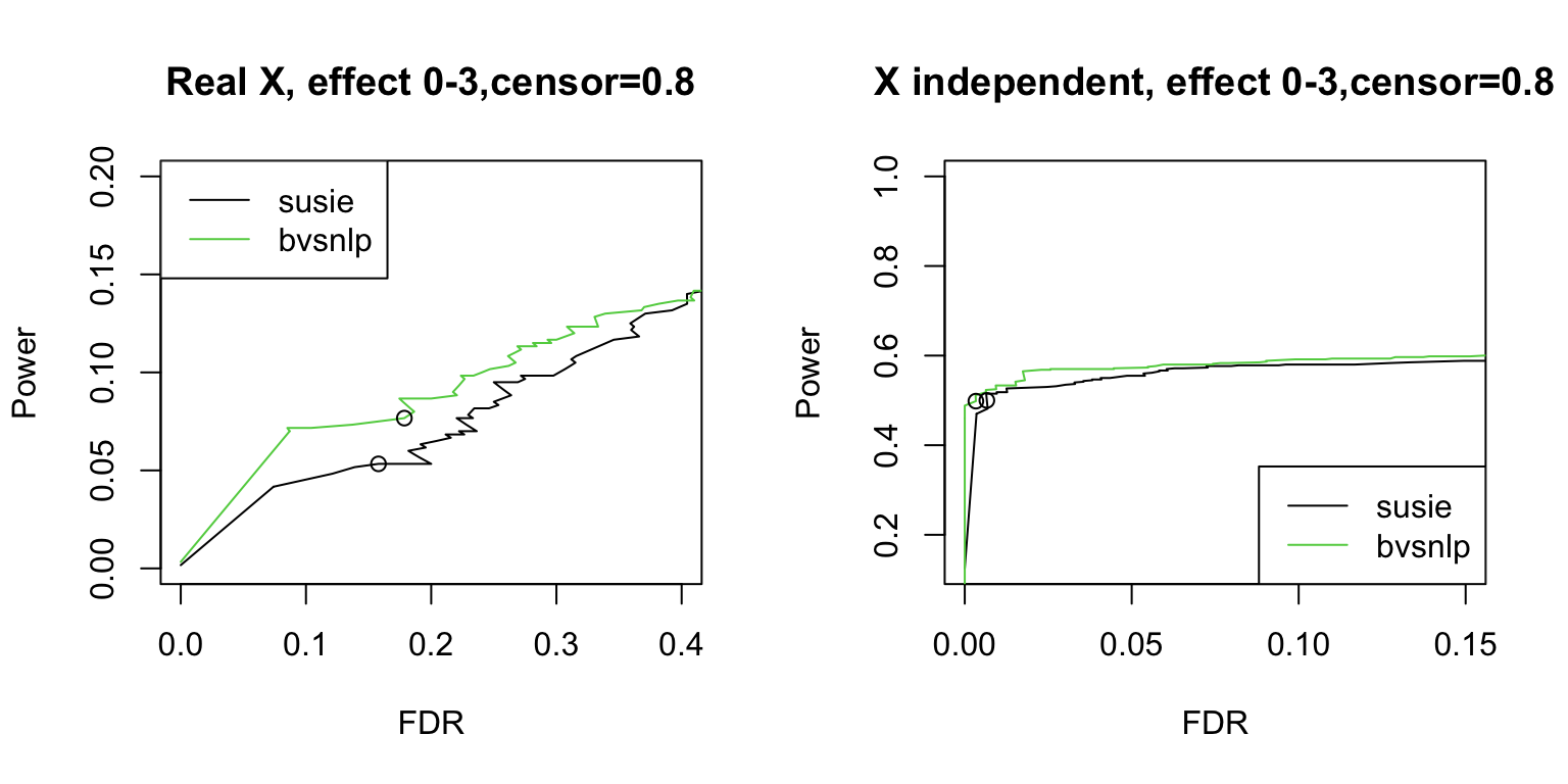
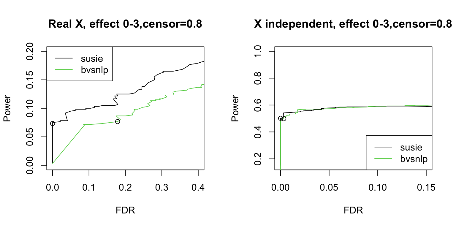
Survival SuSiE vs BVSNLP

A correction to Wakefield’s ABF

Overview

GIBSS requires computing the BF and posterior mean for each variable
Standard statistical software for computing MLE
For large sample sizes, we can leverage asymptotic normality of the MLE to approximate posterior mean and BF.

Posterior mean

\[ \begin{aligned} \hat \beta | \beta, s^2 &\sim N(\beta, s^2) \\ \beta &\sim N(0, \sigma^2) \end{aligned} \]

\[ \beta | \hat \beta, s^2 \sim N \left( \frac{\sigma^2}{s^2 + \sigma^2} \hat\beta, \left(\frac{1}{s^2} + \frac{1}{\sigma^2}\right)^{-1} \right) \]

Approximating the the BF

\[BF = \int \color{red}{\frac{ p(\mathcal {\bf y} | {\bf x}, \beta)}{p({\bf y} | \beta = 0)}} N(\beta | 0, \sigma^2) d\beta\]

Approximate the likelihood ratio in a way that’s easy to integrate

\[ LR(\beta_1, \beta_2) = \frac{p(\mathcal {\bf y} | {\bf x}, \beta)}{p({\bf y} | \beta=0)} \]

Wakefields asymptotic BF

Asymptotically, \(\hat \beta | \beta, s^2 \sim N(\beta, s^2)\). Then

\[ LR(\beta, 0) = \frac{p(y | \hat\beta, \beta) p(\hat\beta | \beta)}{p(y | \hat\beta, \beta = 0) p(\hat\beta | \beta = 0)} \approx \color{red}{\frac{p(y | \hat\beta)}{p(y | \hat\beta)}} \frac{p(\hat\beta | \beta)}{ p(\hat\beta | \beta = 0)} \approx \frac{N(\hat\beta| \beta, s^2)}{N(\hat\beta| 0, s^2)} = \widehat{LR}_{ABF}(\beta, 0). \]

Integrating over the prior gives Wakefield’s asymptotic Bayes Factor (ABF)

\[ ABF = \int \widehat{LR}_{ABF}(\beta, 0) N(\beta | 0, \sigma^2_0) d\beta = \frac{N(\hat\beta | 0, s^2 + \sigma^2_0)}{N(\hat\beta | 0, s^2)} \]

A problem with ABF

\(LR(\beta, 0) \approx \widehat {LR}_{ABF}(\beta, 0)\)
\(LR(0, 0) = \widehat {LR}_{ABF}(0, 0) = 1\)
The asymptotic approximation may not be a good in the tails, an issue for \(\hat\beta/s >> 0\)

Adjusting the ABF

Idea: use the asymptotic approximation where it is good

\[ \begin{aligned} LR(\beta, 0) &= LR(\beta, \hat{\beta}) LR(\hat{\beta}, 0) \\ &\approx \widehat{LR}_{ABF}(\beta, \hat\beta)LR(\hat\beta, 0) \\ &= \widehat{LR}_{Lap}(\hat\beta, 0) \end{aligned} \]

Requires an extra piece of information: \(LR(\hat\beta, 0)\)

Corrected ABF/Laplace approximation

Requires knowledge of the LR of the MLE against the null.
Can dramatically improve approximation of the BF

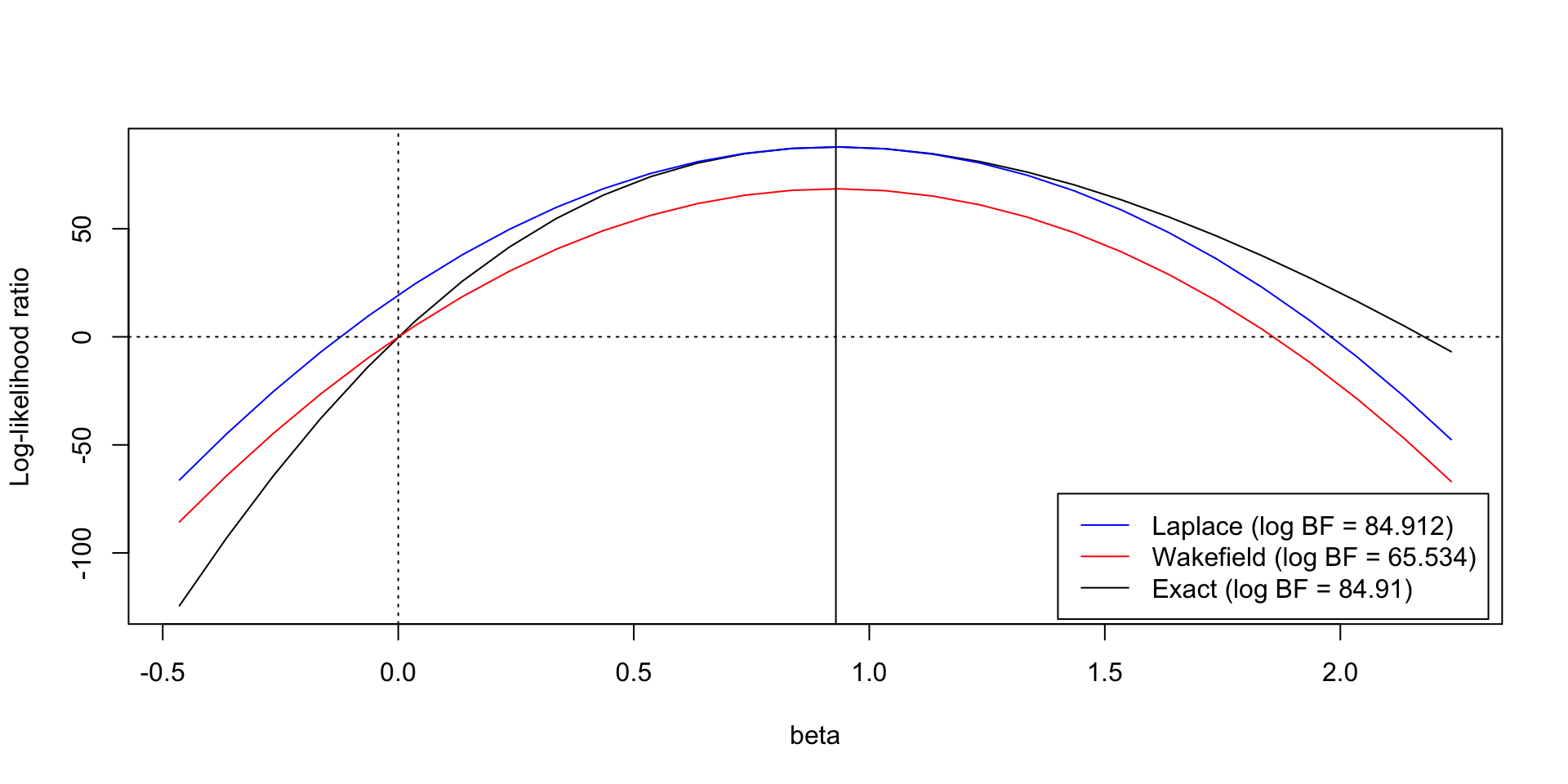
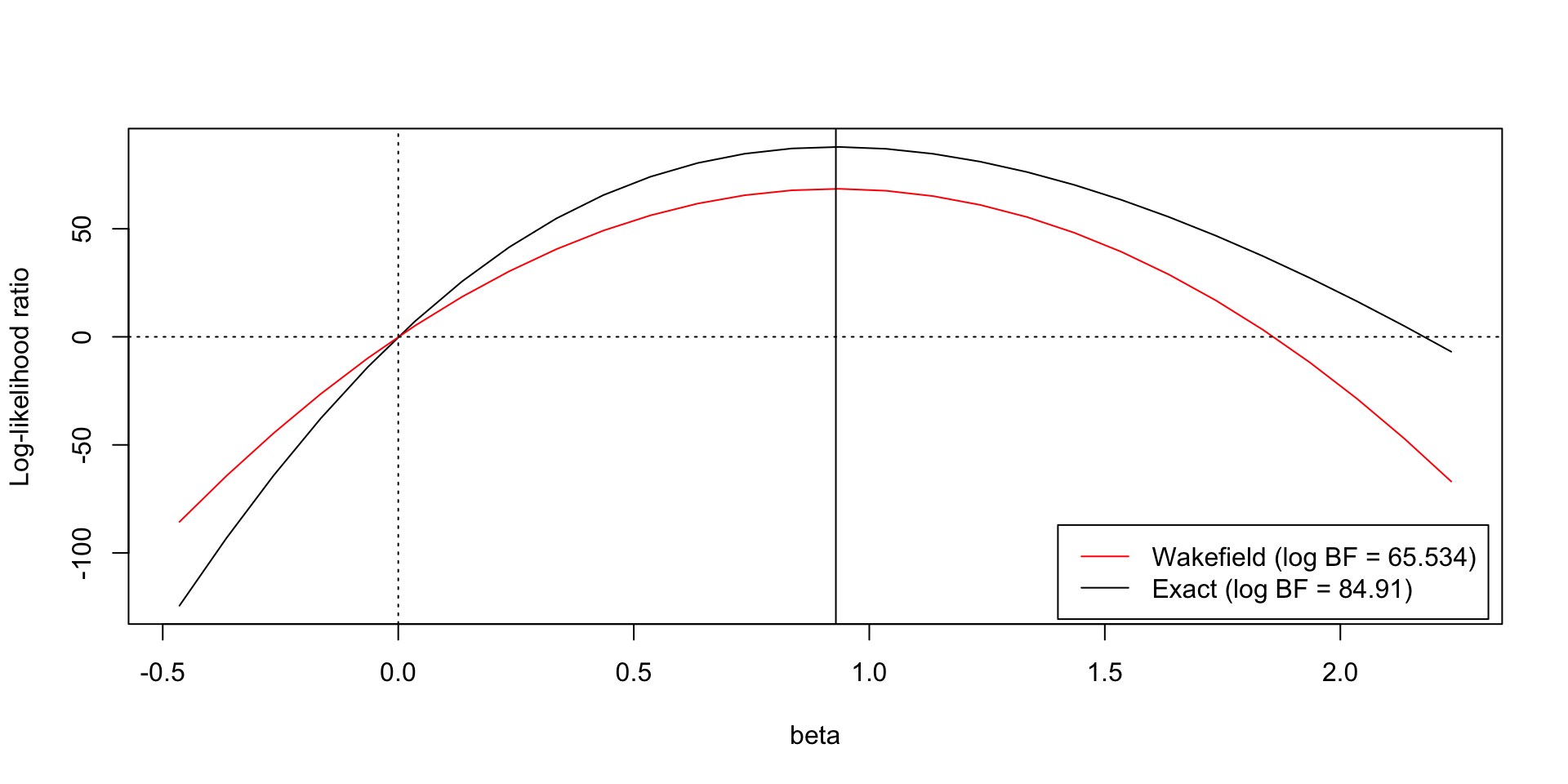
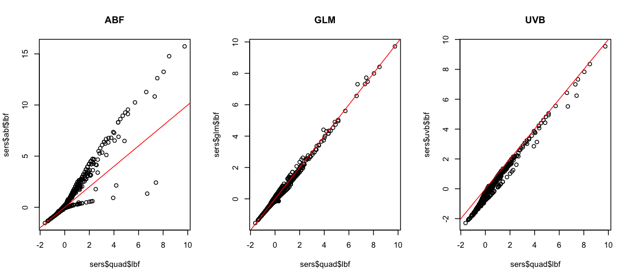
Comparison of logBF

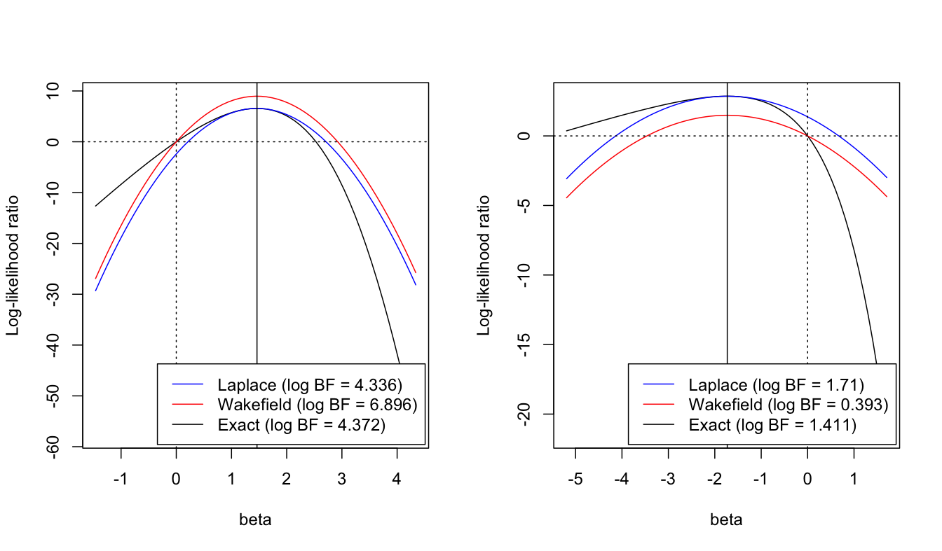
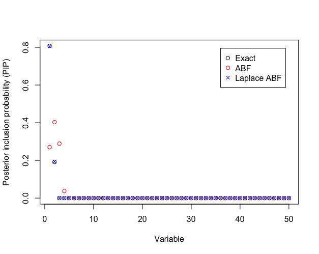
ABF Correction reorders PIPs

Laplace approximation

For some non-negative function \(f: \mathbb R \rightarrow \mathbb R^+\), want to compute the integral

\[I = \int f(x) dx,\]

Define \(h(x) = \log f(x)\), expand around the maximizer of \(h\), \(x^*\)

\[\hat h (x) = h(x^*) + \frac{1}{2} h^{''}(x^*)(x-x^*)^2\]

Approximate with the Gaussian integral

\[ \hat I = \int \exp{\hat h(x))} dx = \exp{\hat h(x^*)} \left(-\frac{2\pi}{h^{''}(x^*)}\right)^{1/2}\] . . .

Potential next step: saddle point approximations?

Takeaways

Laplace approximation of the BF better than ABF for variable selection
Addition information available from standard statistical software for GLMs
Poor performance of ABF raises concerns about using SuSiE-RSS for summary statistics from non-Gaussian models
GIBSS + asymptotic approximation looks like a good recipe for GLMs

Fast implementation

Problem

GIBSS requires evaluating many univariate regression
GLMs fit via IRLS (equivalently, Newton-Raphson with step-size \(\gamma = 1\)). \(\beta_t = \beta_{t-1} - \gamma H^{-1}_{t-1} g_{t-1}\)
\(p\) 2d optimization problems that can be carried out in parallel

Implementation

Implemented in Python using Google’s jax (numpy, with automatic differentiation, JIT compilation, and vectorization)
Newton-Raphson with halving step-size
Easy to extend to many GLMs (or any regression with twice-differentiable log-likelihood)– just define a log_likelihood function.
susiepy package at http://github.com/karltayeb/susiepy

Open questions for optimizing implementation

Coordinate ascent faster on machine compared to full Newton updates?
Avoid fitting intercept for each variable separately?
Avoid checking for likelihood increase
Exploit sparsity in \(X\) for faster implementation?
Partial updates of “inner loop” while fitting GIBBS