Committee Meeting

Karl Tayeb

6/5/23

Aims

A new method for joint gene set enrichment analysis (GSEA)
Joint enrichment models for covariate moderated FDR.
Apply joint enrichment models to increase power in single cell eQTL studies.

Theme: variable selection in non-Gaussian models

Aim 0

Develop general approaches for applying SuSiE to a wide class of non-Gaussian models.

Need good version of logistic SuSiE (and multinomial SuSiE) for GSEA and covariate moderated FDR application (Aim 1 and 2)
We identified serious limitations in our old approach
Two new approaches, both extend beyond the logistic case

SuSiE Basics

Sum of single effects regression (SuSiE)

\({\bf y} \in \mathbb R^n\), \(X \in \mathbb R^{n \times p}\)

Sum of single effects: there are at most \(L\) non-zero effects

\[\begin{align} {\bf y} &\sim N(X\beta, {\bf I}_n \sigma^2) \\ \beta &= \sum_{l=1}^L b_l \gamma_l \\ b_l &\sim N(0, \sigma^2_0) \\ \gamma_l &\sim \text{Multinomial}(1, \pi) \end{align}\]

What makes SuSiE work?

We will quickly review variational inference for SuSiE.

Two key ingredients:

Variational approximation \(q(\beta) = \prod_l q(\beta_l)\)
Gaussian likelihood reduces coordinate updates to solving a SER

Single Effect Regression (SER)

Model

Single effect regression assumes there is exactly one non-zero effect.

\({\bf y} \in \mathbb R^n\), \(X \in \mathbb R^{n \times p}\) \[ \begin{aligned} {\bf y} &\sim N(X\beta, {\bf I}_p \sigma^2_0) \\ \beta &= b \gamma \\ b &\sim N(0, \sigma^2_0)\\ \gamma &\sim \text{Multinomial}(1, \pi) \end{aligned} \]

Inference is easy

Compute the posterior for \(j = 1,\dots , p\) separate univariate regression \[p(b | X, {\bf y}, \gamma_j = 1)\]
Compute posterior inclusion probabilities

\[ p(\gamma_j = 1 | {\bf y}, X) \propto BF_j \pi_j \]

\[ BF_j = \frac{p({\bf y} | X, \gamma_j=1 )}{p({\bf y} | \beta=0)} \]

Variational inference

Inference as an optimization problem:

\[\begin{align} p(\beta | {\bf y}, X) = \arg \max_q F(q), \quad F(q) := \mathbb E_q \left[ \log p ({\bf y} | X, \beta) \right] - KL[q || p] \end{align}\]

\[\begin{align} F(q) &= \mathbb E_q \left[ \log p ({\bf y} | X, \beta) \right] - KL[q || p] \\ &= \mathbb E_q \left[ \log p ({\bf y}, \beta | X) \right] + H(q) \\ &= \left(\mathbb E_q \left[ \log p ({\bf y}, \beta | X) - Z \right] + H(q) \right) + Z \\ &= - KL[q || p_{post}] + Z \end{align}\]

We’ll write the variational objective for SER \(F_{SER}(q; {\bf y}, X, \sigma_0)\)

SuSiE: model

\[ \begin{aligned} y &\sim N(X\beta, \sigma^2_0) \\ \beta &= \sum_l b_l \gamma_l \\ b_l &\sim N(0, \sigma^2_0)\\ \gamma_l &\sim \text{Multinomial}(1, \pi) \end{aligned} \]

SuSiE: variational approximation

Restrict \(q\) to some family \(\mathcal Q\)

\[\begin{align} q^*(\beta) = \arg \max_{q \in \mathcal Q} F(q) \end{align}\]

SuSiE uses \(\mathcal Q = \{q : q(\beta) = \prod_l q_l(\beta_l)\}\)

\[ F_{SuSiE}(q; X, {\bf y}) = \mathbb E_{q} \left[ -\frac{1}{2\sigma^2}||{\bf y} - {\bf X} \beta_{-l} - X\beta_l||^2_2) \right] + KL[q || p_{SuSiE}] \]

SuSiE: coordinate ascent (IBSS)

Define the residual \({\bf r}_l = {\bf y} - X\beta_{-l}\)

\[ \begin{aligned} F_{SuSiE}(q_l; q_{-l}, X, {\bf y}) &= \mathbb E_{q_l} \left[ \mathbb E_{q_{-l}} \left[ -\frac{1}{2\sigma^2}||{\bf y} - {\bf X} \beta_{-l} - X\beta_l||^2_2) \right] \right] - KL[q || p] \\ &= \mathbb E_{q_l} \left[ \mathbb E_{q_{-l}} \left[ -\frac{1}{2\sigma^2}|| {\bf r}_l - X\beta_l||^2_2) \right] \right] - KL[q_l || p_l] + C_1 \\ &= \mathbb E_{q_l} \left[ \color{blue}{ -\frac{1}{2\sigma^2} \left(|| \mathbb E_{q_{-l}} {\bf r}_l- X\beta_l||^2_2 + \mathbb V ||r_l||^2_2 \right)} \right] - KL[q_l || p_l] + C_1\\ &= \mathbb E_{q_l} \left[ -\frac{1}{2\sigma^2} || \mathbb E_{q_{-l}} {\bf r}_l- X\beta_l||^2_2] \right] - KL[q_l || p_l] + C_2 \\ &= F_{SER}(q_l; X, \mathbb E_{q{-l}}{\bf r}_l) + C_2 \end{aligned} \]

Key: coordinate updates in \(\mathcal Q\) reduce to solving an SER

Generalizing SuSiE

Simplification depends on properties of the Gaussian log likelihood

\[ \begin{aligned} \log p(y | {\bf x}, \beta) = y ({\bf x}^T \beta) - \log(1 + \exp({\bf x}^T \beta)) \end{aligned} \]

No simplification when taking expectations over \(q_{-l}\)

\[ \begin{aligned} \mathbb E_{q_{-l}} \left[ \log p(y | {\bf x}, \beta) \right] = y ({\bf x}^T \beta_l + {\bf x}^T \bar \beta_{-l}) - \color{red}{\mathbb E_{q_{-l}}\left[\log(1 + \exp({\bf x}^T \beta)) \right]} \end{aligned} \]

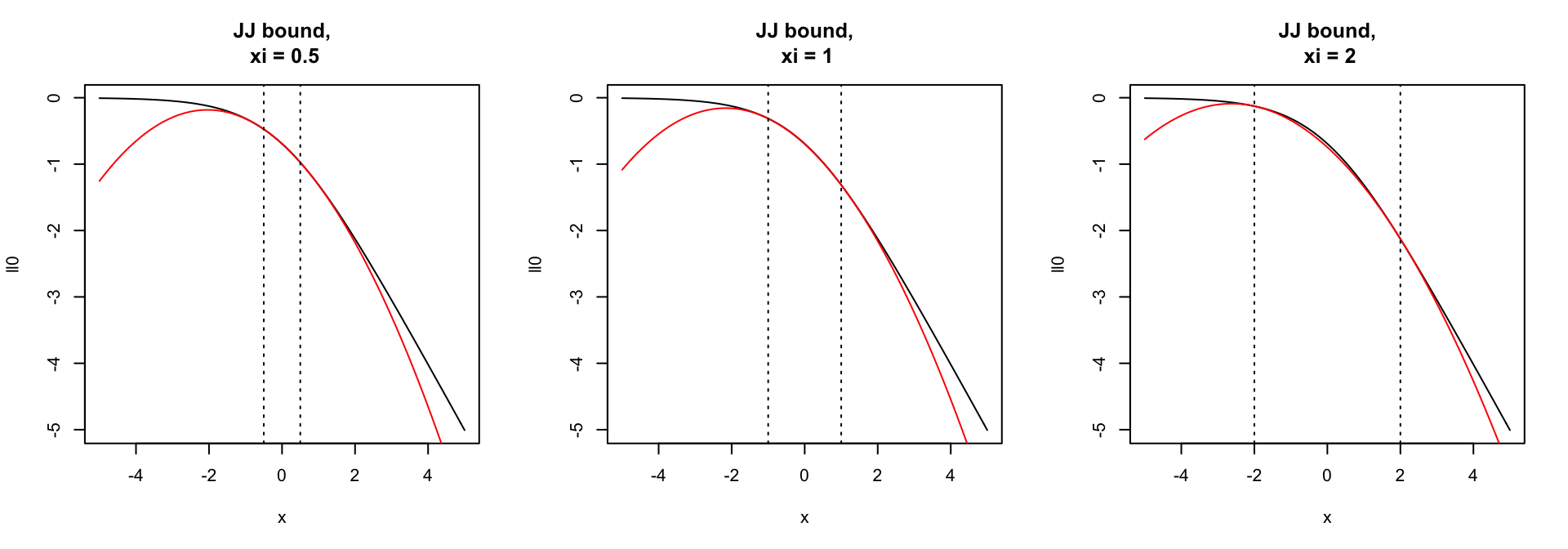
Jaakkola-Jordan bound

Idea: construct local approximation to the log-likelihood. Tune the approximation to be tight near the posterior mode.

For all \(\xi \in \mathbb R\), \(\psi = {\bf x}^T \beta\)

\[ \log p(y | \psi) \geq \frac{1}{2} \log \sigma(\xi) + \frac{1}{2} \left((2y -1) \psi - \xi\right) - \frac{1}{4\xi}\tanh(\frac{\xi}{2}) (\psi^2 - \xi^2) \]

JJ Bound is bad for variable selection

Naive application of JJ bound to SER uses very loose ELBO for most variables

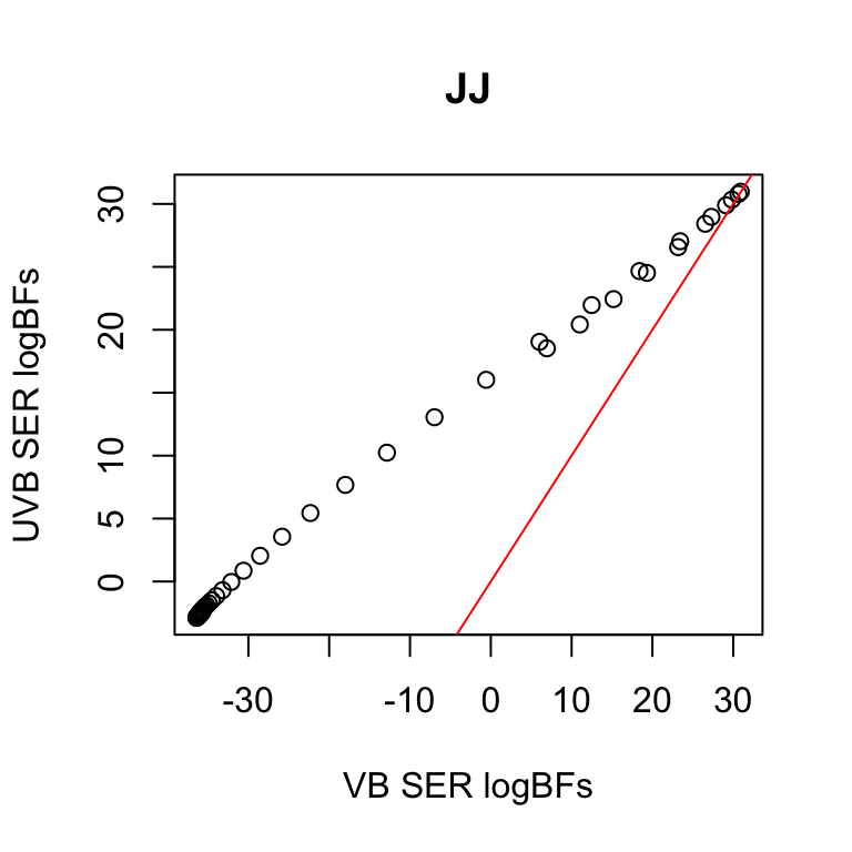
Winner take all: Coverage of 90% credible sets across 1k SER simulations
method	coverage
uvb_ser	0.945
vb_ser	0.845

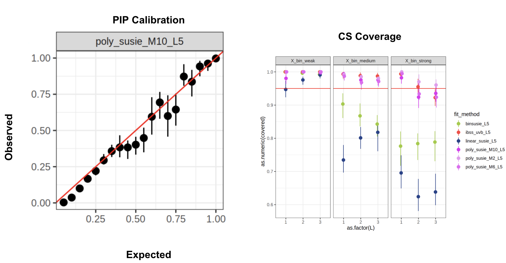
Simulations: VB logistic SuSiE \(L=5\)

Varying effect sizes, correlation structure, and num. of non-zero effects

Generalized IBSS

Overview

Heuristic approach for applying SuSiE to non-Gaussian models
Idea: apply IBSS, using expected predictions as fixed offsets

\[\begin{align} F_{SuSiE}(q) &= \mathbb E_q[\log p({\bf y} | X, \beta_l, \beta_{-l})] - \sum_l KL[q_l || p_l] \\ &= \mathbb E_{q_l}[ \mathbb E_{q_{-l}}[\log p({\bf y} | X, \beta_l, \beta_{-l})]] - \sum_l KL[q_l || p_l] + C_1 \\ &\color{purple}{\approx \mathbb E_{q_l}[\log p({\bf y} | X, \beta_l, \bar \beta_{-l})] - KL[q_l || p_l] + C_2} \\ &= F_{SER}(q_l; {\bf y}, X, \bar \beta_{-l}) + C_2 \end{align}\]

Why should this work?

\[\begin{align} F_{SuSiE}(q) &= \mathbb E_q[\log p({\bf y} | X, \beta_l, \beta_{-l})] - \sum_l KL[q_l || p_l] \\ &\color{purple}{\approx \mathbb E_{q_l}[\log p({\bf y} | X, \beta_l, \bar \beta_{-l})] - KL[q_l || p_l] + C_2} \\ \end{align}\]

If \(\log p( {\bf y} | X, \beta)\) is quadratic in \(\beta\) (Gaussian) there \(\color{purple}\approx\) is \(=\)
Informally, approximation is good if \(\log p( {\bf y} | X, \beta)\) is well approximated by a quadratic function in \(\beta\).
Really we care about \(\psi = X\beta\)

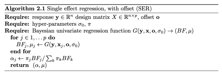
Algorithm: Single effect regression

Require a function \(G\) which computes the BF and posterior mean of a Bayesian univariate regression

\[\begin{align} {\bf y} \sim 1 + {\bf x} + {\bf o} \\ b \sim N(0, \sigma^2) \end{align}\]

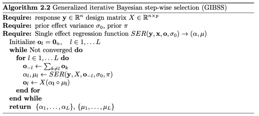
Algorithm: GIBSS

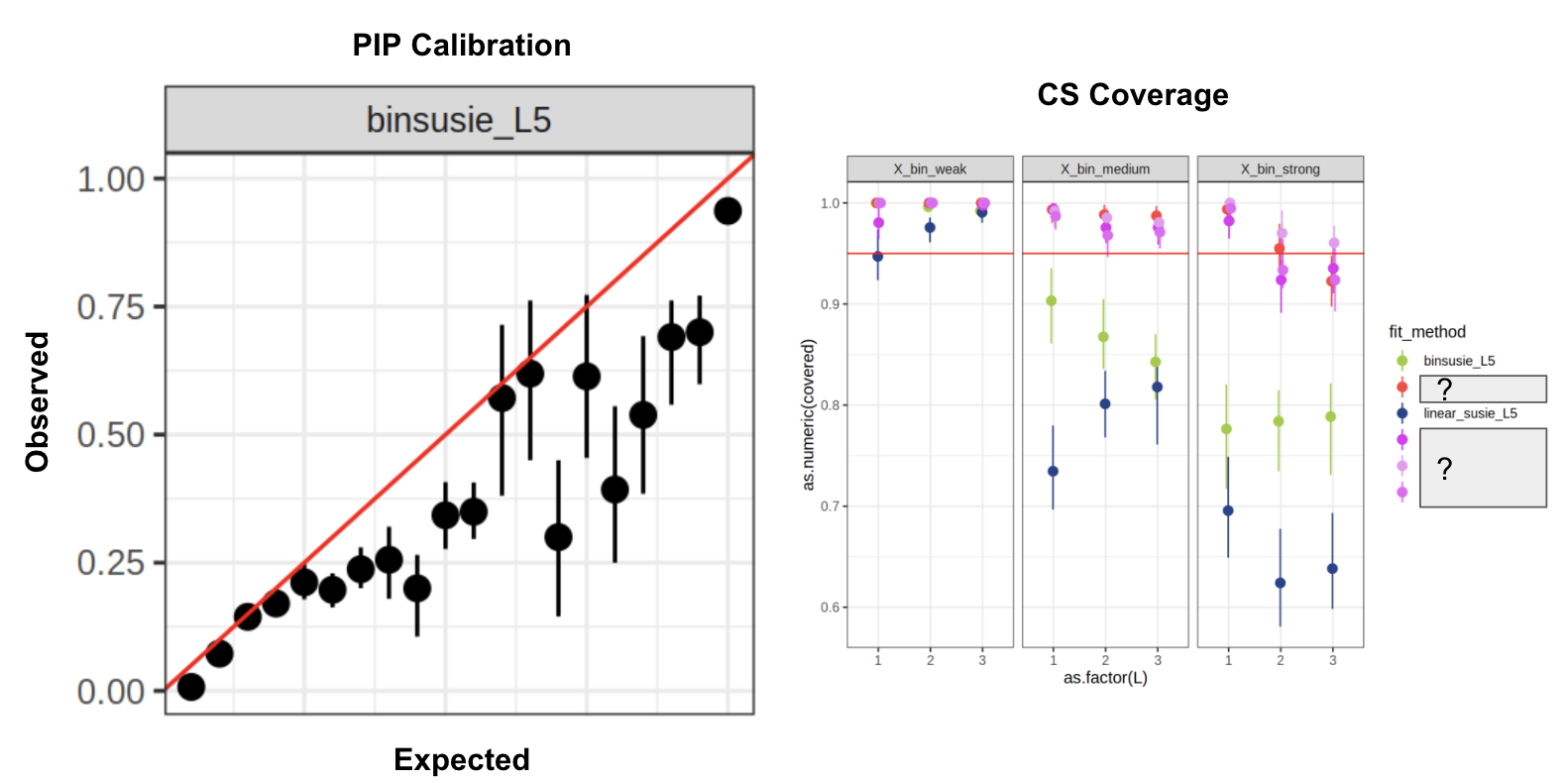
Simulations: logistic-GIBSS \(L=5\)

Much better performance compared to direct VB approach

Advantage and limitations

Advantages

Seems to work well!
Highly modular: just need to implement the univariate regression

Disadvantages

Heuristic– not optimizing a clear objective function
Does not properly account for uncertainty in \(\beta_{-l}\), only uses posterior mean

Opportunities

Can we analyze the approximation error?
Can we make guarantees on GIBSS performance asymptotically?

Status

Implemented in logisticsusie package github rep
Yunqi was able to use GIBSS code to help with survival SuSiE project
Possibly implement GIBSS for GLMs in susieR package

A correction to Wakefield’s ABF

Overview

GIBSS requires computing the BF and posterior mean for each variable
Standard statistical software for computing MLE
For large sample sizes, we can leverage asymptotic normality of the MLE to approximate posterior mean and BF.

Posterior mean

\[ \begin{aligned} \hat \beta | \beta, s^2 &\sim N(\beta, s^2) \\ \beta &\sim N(0, \sigma^2) \end{aligned} \]

\[ \beta | \hat \beta, s^2 \sim N \left( \frac{\sigma^2}{s^2 + \sigma^2} \hat\beta, \left(\frac{1}{s^2} + \frac{1}{\sigma^2}\right)^{-1} \right) \]

Approximating the the BF

\[BF = \int \color{red}{\frac{ p(\mathcal {\bf y} | {\bf x}, \beta)}{p({\bf y} | \beta = 0)}} N(\beta | 0, \sigma^2) d\beta\]

Approximate the likelihood ratio in a way that’s easy to integrate

\[ LR(\beta_1, \beta_2) = \frac{p(\mathcal {\bf y} | {\bf x}, \beta)}{p({\bf y} | \beta=0)} \]

Wakefields asymptotic BF

Asymptotically, \(\hat \beta | \beta, s^2 \sim N(\beta, s^2)\). Then

\[ LR(\beta, 0) = \frac{p(y | \hat\beta, \beta) p(\hat\beta | \beta)}{p(y | \hat\beta, \beta = 0) p(\hat\beta | \beta = 0)} \approx \color{red}{\frac{p(y | \hat\beta)}{p(y | \hat\beta)}} \frac{p(\hat\beta | \beta)}{ p(\hat\beta | \beta = 0)} \approx \frac{N(\hat\beta| \beta, s^2)}{N(\hat\beta| 0, s^2)} = \widehat{LR}_{ABF}(\beta, 0). \]

Integrating over the prior gives Wakefield’s asymptotic Bayes Factor (ABF)

\[ ABF = \int \widehat{LR}_{ABF}(\beta, 0) N(\beta | 0, \sigma^2_0) d\beta = \frac{N(\hat\beta | 0, s^2 + \sigma^2_0)}{N(\hat\beta | 0, s^2)} \]

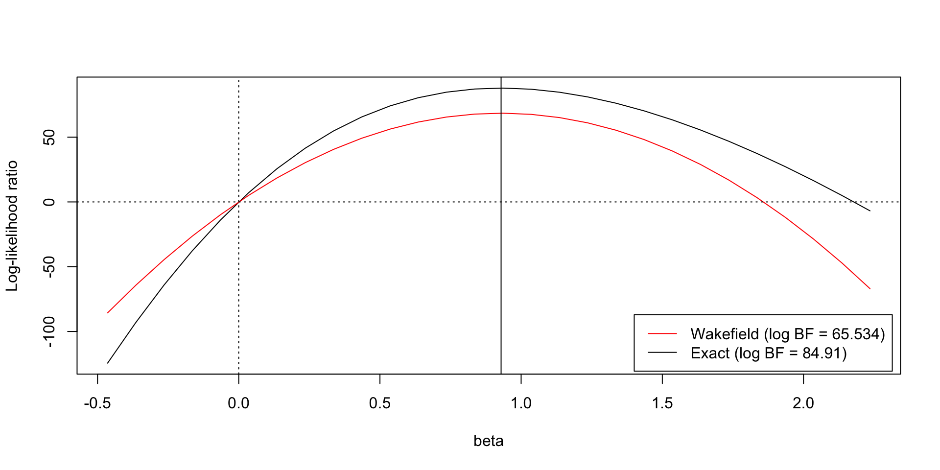
A problem with ABF

The asymptotic approximation may not be a good in the tails
An issue for \(\hat\beta/s >> 0\)

Adjusting the ABF

Idea: use the asymptotic approximation where it is good

\[ \begin{aligned} LR(\beta, 0) &= LR(\beta, \hat\beta) LR(\hat\beta, 0) \\ &\approx \widehat{LR}_{ABF}(\beta, \hat\beta)LR(\hat\beta, 0) \\ &= \widehat{LR}_{Lap}(\hat\beta, 0) \end{aligned} \]

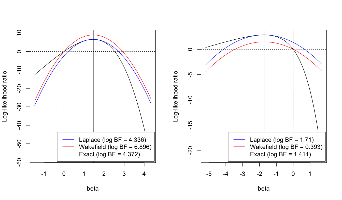
Corrected ABF/Laplace approximation

Requires knowledge of the LR of the MLE against the null.
Can dramatically improve approximation of the BF

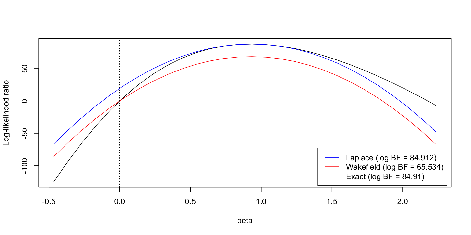
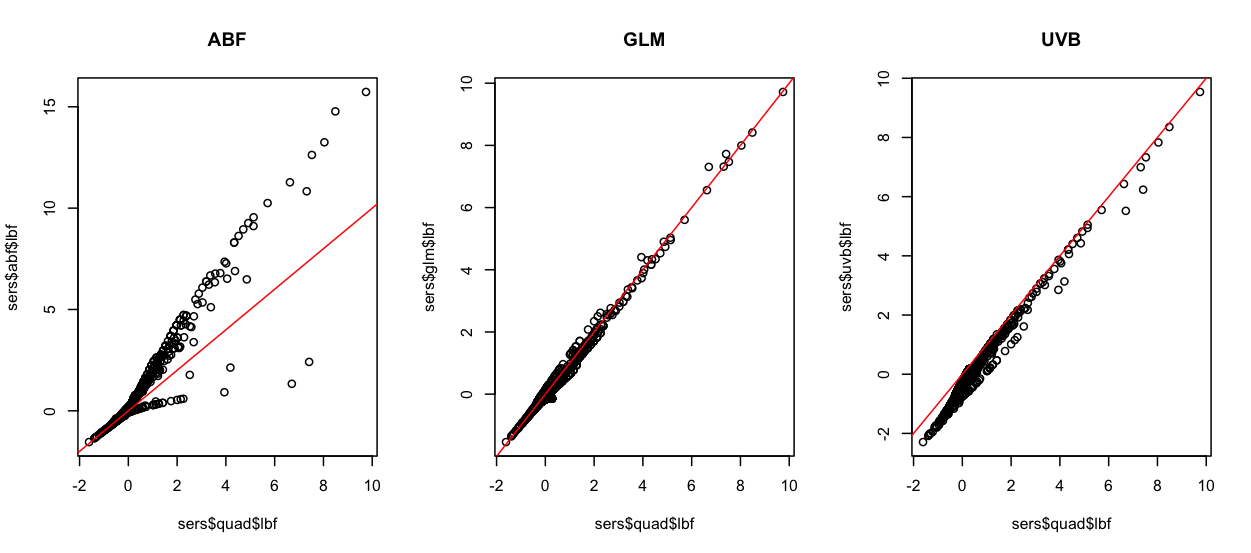
Comparison of logBF

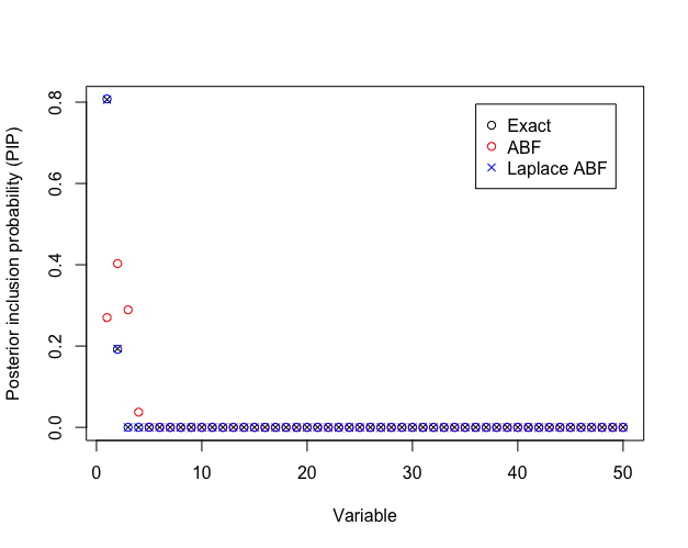
ABF Correction reorders PIPs

Laplace approximation

For some non-negative function \(f: \mathbb R \rightarrow \mathbb R^+\), want to compute the integral

\[I = \int f(x) dx,\]

Define \(h(x) = \log f(x)\), expand around the maximizer of \(h\), \(x^*\)

\[\hat h (x) = h(x^*) + \frac{1}{2} h^{''}(x^*)(x-x^*)^2\]

Approximate with the Gaussian integral

\[ \hat I = \int \exp{\hat h(x))} dx = \exp{\hat h(x^*)} \left(-\frac{2\pi}{h^{''}(x^*)}\right)^{1/2}\]

Takeaways

Laplace approximation of the BF better than ABF for variable selection
Addition information available from standard statistical software for GLMs
Poor performance of ABF raises concerns about using SuSiE-RSS for summary statistics from non-Gaussian models
GIBSS + asymptotic approximation looks like a good recipe for GLMs

Polynomial SuSiE

Notation

\(p\) an \(M\) degree polynomial

\({\bf a} = (a_0, \dots, a_M)\) unique coefficients representing \(p\) in the monomial basis \((1, x, \dots, x^M)\)

\[\phi_{\bf a}(x) = \sum_{k=0}^M a_k x^k = p(x)\]

Polynomial approximation: inference

Approximate the log-likelihood of each observation as a polynomial in linear prediction, \(\psi\). \({\bf a}_i\) s.t. \(\log p(y_i | \psi) \approx \phi_{{\bf a}_i}(\psi)\)
Approximate the log prior density. \(\rho\) s.t. \(\log p(\beta) \approx \phi_{\rho}\)
Transform \({\bf a}_i\) so they are a function of \(\beta\). \({\bf d}_i\)
\(\log p(y, \beta) \approx \phi_{\bf f}(\beta), \quad {\bf f} := \sum {\bf d_i} + \rho\)

Polynomial exponential family

With \({\bf a} \in \mathbb R^M\), and \(T(x) = (x, \dots, x^M)\)

\[ f(x; {\bf a}) \propto \exp\{\langle {\bf a}, T(x) \rangle\} \]

Intercept = normalizing constant. \(a_0 = - \log \int \exp\{\langle {\bf a}, T(x) \rangle\} dx\)
Hard integral, approximate or handle numerically

Operations: polynomial rescaling

\[\phi_{\bf a}(cx) = \phi_{{\bf d}({\bf a}, c)}(x)\]

\[ \begin{aligned} \sum_m a_m(c x)^m &= \sum_m (a_m c^m) x^m \\ &= \sum_m {\bf d}({\bf a}, c)_m x^m, \quad {\bf d}({\bf a}, c)_m := a_mc^m \end{aligned} \]

Polynomial approximate univariate regression

For each \(i\), we have \({\bf a}_i\) such that \(\log p(y_i | \psi) \approx \phi_{{\bf a}_i}(\psi)\)
Represent/approximate the log-prior density with a polynomial with coefficients \(\rho\), i.e. \(\log p(\beta) \approx \phi_\rho(\beta)\)

\[\begin{align} \log p({\bf y}, \beta | {\bf x}, \beta) &\approx \sum_i \phi_{{\bf a}_i}(x_i \beta) + \phi_{\rho}(\beta)\\ &= \sum_i \phi_{{\bf d}({\bf a}_i, x_i)}(\beta) + \phi_{\rho}(\beta) \\ &= \phi_{{\bf f}(A, {\bf x}, \rho)}(\beta), \quad {\bf f}(A, {\bf x}, \rho) = \sum_i {\bf d}({\bf a}_i, x_i) + \rho \end{align}\]

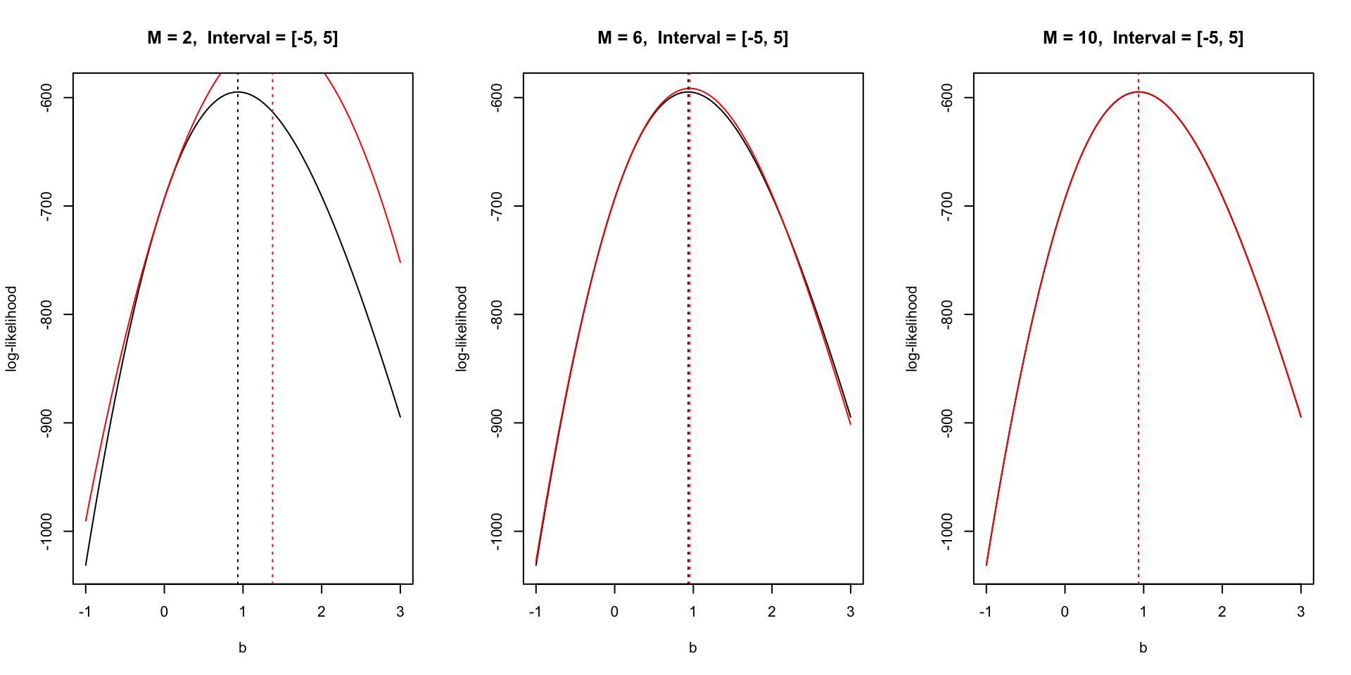
Example: univariate regression

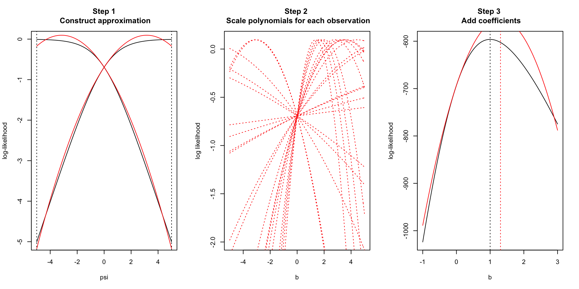
Increasing degree increases accuracy

Polynomial SER

\(A = \{{\bf a}_i \}_{i=1}^n\), base coefficients

\[ \hat F_{SER}(q; A, X, \sigma^2_0) = \mathbb E_q\left[ \sum \phi_{{\bf a}_i}(\psi_i)]\right] - KL[q || p] \approx F_{SER}(q; {\bf y}, X, \sigma^2_0). \]

Approximate the SER by exactly optimizing an approximation of the ELBO
Each univariate regression is easy to compute from the base coefficient \(A\)

Operations: polynomial shift

For SuSiE: \(\psi = \psi_l + \psi_{-l}\).

\[\phi_{\bf a}(x + y) = \phi_{{\bf b}({\bf a}, y)}(x)\]

Expand and collect terms

\[\begin{align} \phi_{\bf a}(x + y) &= \sum_{m=0}^M a_m(x + y)^m = \sum_{m=0}^M a_m \sum_{k=0}^m {m \choose k} x^k y^{m-k} \\ &= \sum_{k=0}^M \left(\sum_{m=k}^M a_m {m \choose k}y^{m-k} \right) x^k \\ &= \sum_{k=0}^M {\bf b}({\bf a}, y)_k x^k, \quad {\bf b}({\bf a}, y)_k := \left(\sum_{m=k}^M a_m {m \choose k}y^{m-k} \right) \end{align}\]

Can be written as a matrix multiplication \[ {\bf b}({\bf a}, y) = M(y) {\bf a}, \quad M_{ij} = {j \choose i} y^{j -i}\; \forall j \geq i, 0 \text{ otherwise} \]

For random \(y \sim p\), expected polynomial shift

\[ {\bf c}({\bf a}, p) := \mathbb E_p[{\bf b}({\bf a}, y)] = \mathcal M(p){\bf a}, \quad \mathcal M(p) := \mathbb E_p[M(y)] \]

Polynomial shift for SuSiE

Each observation must be transformed into a function of \(\psi_{l}\)

Start with \({\bf a}^* = \mathcal M(q){\bf a}\)

“Undo” polynomial shift \({\bf a}^{(l)} = M(q_l)^{-1} {\bf a}^*\)
Update \(q_{l, new} \leftarrow \arg\max_{q_l}\hat F_{SER}(q_l; A^{(l)}, X, \sigma^2_0)\)
\({\bf a}^*_{new} \leftarrow \mathcal M(q_{l, new}) {\bf a}^{(l)}\)

The SER coefficients \({\bf a}^{(l)}\) analogous to expected residuals in IBSS
\(\mathcal M(q_l)\) requires \(\mathbb E_{q_l}\left[\psi^k\right], \; k = 1, \dots M\)

Coordinate ascent in an variational objective

\[\begin{align} \hat F_{SuSiE}(q_l; q_{-l}, A, X, \sigma^2_0) &= \mathbb E_{q_l} \mathbb E_{q_{-l}} \sum_i \phi_{{\bf a}_i}(\psi_l + \psi_{-l}) + KL[q|| p] \\ &= \mathbb E_{q_l} \mathbb E_{q_{-l}} \sum_i \phi_{{\bf c}({\bf a}_i, \psi_{-l})}(\psi_l) + KL[q_l|| p_l] + C \\ &= \mathbb E_{q_l} \sum_i \phi_{{\bf d}({\bf a}_i,q_{-l})}(\psi_l) + KL[q_l|| p_l] + C \\ &= \hat F_{SER} (q_l; D, X, \sigma^2_0) + C, \quad D = \{{\bf d}({\bf a}_i,q_{-l})\}_{i=1}^n \end{align}\]

Polynomial interpolation

\(f : \mathbb R \rightarrow \mathbb R\)

\(n+1\) distinct points \(x_0 < \dots < x_{n}\)

There exists a unique \(p \in P_n\) such that \(p\) interpolates \(f\) at \(x_0, \dots, x_n\).

\[\begin{align} p(x) = \sum_{i=0}^n f(x_i) L_{n, i}(x), \quad L_{n, i}(x) = \prod_{k \neq i} \frac{x - x_k}{x_i - x_k} \end{align}\]

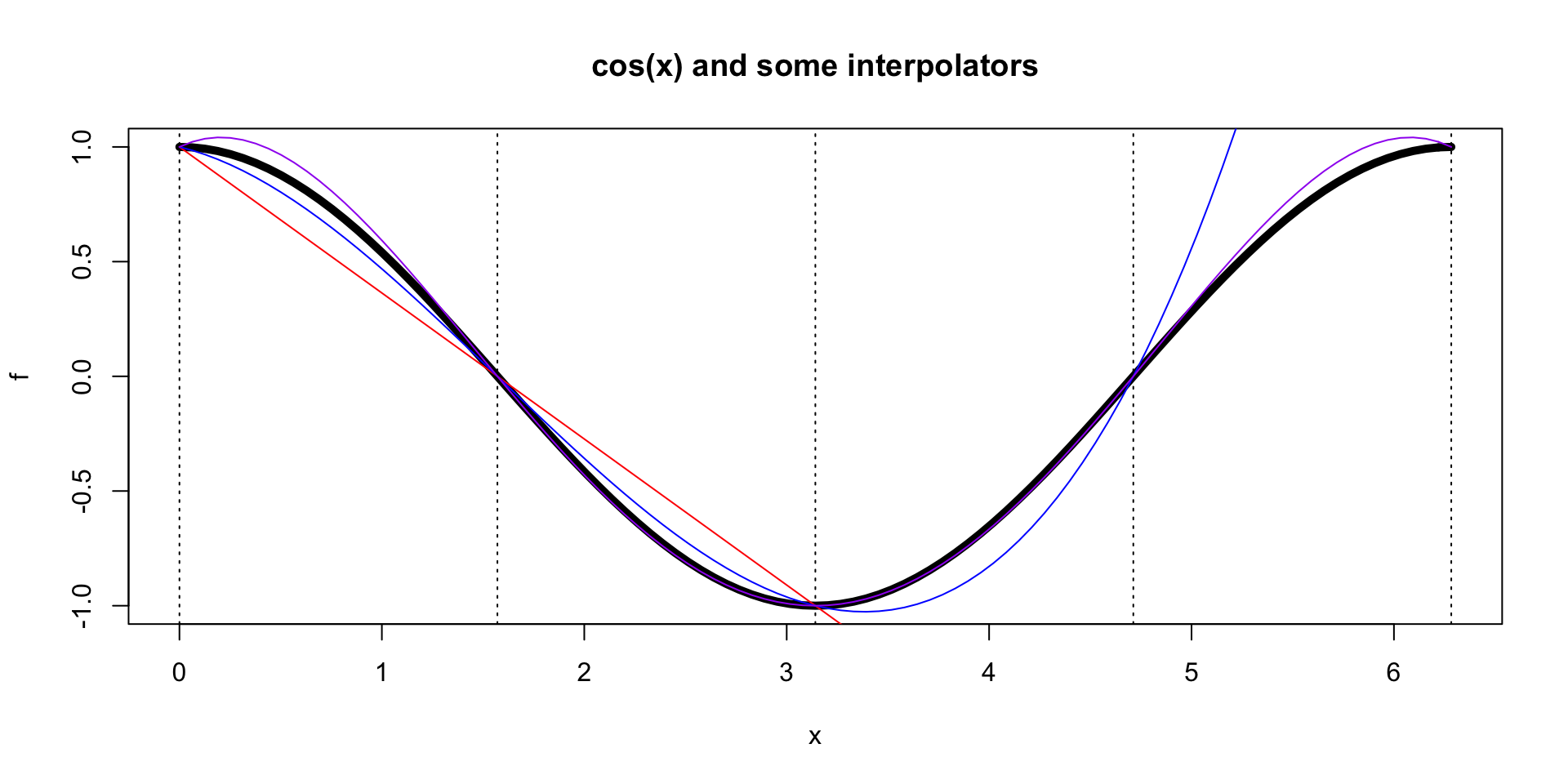
Chebyshev interpolation

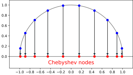
Interpolation at the zeros of Chebyshev polynomials \(x_k = \cos \left(\frac{2k-1}{2M}\pi \right), k = 1, \dots, M\)
Fast interpolation via re-scaled DFT of \(f(x_1), \dots, f(x_M)\)
Approximately minimizes \(||f - \hat f||_{\infty}\)

Chebyshev interpolation: GLM likelihoods

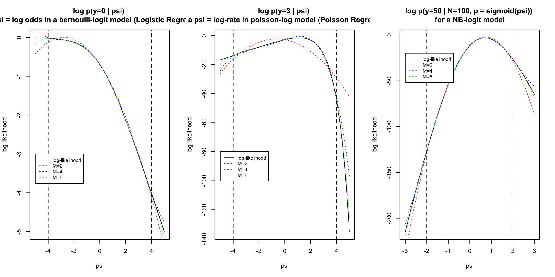
Simulations

Caveats: designing good polynomial approximations

Require the leading degree of the polynomial approximation to be negative so that \(\int \exp \phi_{\bf a} < \infty\)
Approximation interval should contain the prediction for each observation with high probability for the approximation to be accurate \(\mathbb P( \beta^T {\bf x}_i \in [L, R] | {\bf y}, X) \approx 1\)
Quality of the approximation (generally) decreases as approximation interval becomes wider

Opportunities

Is there a faster way to perform “expected polynomial shift” operation?
Other computationally convenient ways to approximation \(\log p(y | \psi)\)?