Getting started
karltayeb
2022-05-16
Last updated: 2022-09-01
Checks: 7 0
Knit directory: logistic-susie-gsea/
This reproducible R Markdown analysis was created with workflowr (version 1.7.0). The Checks tab describes the reproducibility checks that were applied when the results were created. The Past versions tab lists the development history.
Great! Since the R Markdown file has been committed to the Git repository, you know the exact version of the code that produced these results.
Great job! The global environment was empty. Objects defined in the global environment can affect the analysis in your R Markdown file in unknown ways. For reproduciblity it’s best to always run the code in an empty environment.
The command set.seed(20220105) was run prior to running
the code in the R Markdown file. Setting a seed ensures that any results
that rely on randomness, e.g. subsampling or permutations, are
reproducible.
Great job! Recording the operating system, R version, and package versions is critical for reproducibility.
Nice! There were no cached chunks for this analysis, so you can be confident that you successfully produced the results during this run.
Great job! Using relative paths to the files within your workflowr project makes it easier to run your code on other machines.
Great! You are using Git for version control. Tracking code development and connecting the code version to the results is critical for reproducibility.
The results in this page were generated with repository version 753780d. See the Past versions tab to see a history of the changes made to the R Markdown and HTML files.
Note that you need to be careful to ensure that all relevant files for
the analysis have been committed to Git prior to generating the results
(you can use wflow_publish or
wflow_git_commit). workflowr only checks the R Markdown
file, but you know if there are other scripts or data files that it
depends on. Below is the status of the Git repository when the results
were generated:
Ignored files:
    Ignored:    .DS_Store
    Ignored:    .RData
    Ignored:    .Rhistory
    Ignored:    .Rproj.user/
    Ignored:    _targets.R
    Ignored:    _targets.html
    Ignored:    _targets.md
    Ignored:    _targets/objects/
    Ignored:    _targets/user/
    Ignored:    _targets/workspaces/
    Ignored:    _targets_r/
    Ignored:    cache/
    Ignored:    data/.DS_Store
    Ignored:    data/adipose_2yr_topsnp.txt
    Ignored:    data/anthony/
    Ignored:    data/de-droplet/
    Ignored:    data/de-microplastics/
    Ignored:    data/deng/
    Ignored:    data/fetal_reference_cellid_gene_sets.RData
    Ignored:    data/human_chimp_eb/
    Ignored:    data/pbmc-purified/
    Ignored:    data/wenhe_baboon_diet/
    Ignored:    data/yusha_sc_tumor/
    Ignored:    library/
    Ignored:    renv/
    Ignored:    staging/

Untracked files:
    Untracked:  .ipynb_checkpoints/
    Untracked:  Master's Paper.pdf
    Untracked:  Project_1652928411/
    Untracked:  Project_1653228324/
    Untracked:  Project_1653228355/
    Untracked:  VEB_Boost_Proposal_Write_Up (1).pdf
    Untracked:  _targets/meta/
    Untracked:  additive.l5.gonr.aggregate.scores
    Untracked:  analysis/alpha_ash_v_point_normal.Rmd
    Untracked:  analysis/compare_w_post_hoc_clustering.Rmd
    Untracked:  analysis/de_droplet_noshrink.Rmd
    Untracked:  analysis/de_droplet_noshrink_logistic_susie.Rmd
    Untracked:  analysis/fetal_reference_cellid_gsea.Rmd
    Untracked:  analysis/fixed_intercept.Rmd
    Untracked:  analysis/gsea_made_simple.Rmd
    Untracked:  analysis/iDEA_examples.Rmd
    Untracked:  analysis/latent_gene_list.Rmd
    Untracked:  analysis/linear_method_failure_modes.Rmd
    Untracked:  analysis/linear_regression_failure_regime.Rmd
    Untracked:  analysis/linear_v_logistic_pbmc.Rmd
    Untracked:  analysis/logistic_susie_veb_boost_vs_vb.Rmd
    Untracked:  analysis/logistic_susie_vis.Rmd
    Untracked:  analysis/logistic_variational_bound.Rmd
    Untracked:  analysis/logsitic_susie_template.Rmd
    Untracked:  analysis/normal_means.Rmd
    Untracked:  analysis/pcb_scratch.Rmd
    Untracked:  analysis/references.bib
    Untracked:  analysis/roadmap.Rmd
    Untracked:  analysis/sc_tumor_followup.Rmd
    Untracked:  analysis/simulations.Rmd
    Untracked:  analysis/simulations_l1.Rmd
    Untracked:  analysis/tccm_vs_logistic_susie.Rmd
    Untracked:  analysis/template.Rmd
    Untracked:  analysis/test.Rmd
    Untracked:  build_site.R
    Untracked:  code/html_tables.R
    Untracked:  code/latent_logistic_susie.R
    Untracked:  code/logistic_susie_data_driver.R
    Untracked:  code/marginal_sumstat_gsea_collapsed.R
    Untracked:  code/point_normal.R
    Untracked:  code/sumstat_gsea.py
    Untracked:  code/susie_gsea_queries.R
    Untracked:  docs.zip
    Untracked:  export/
    Untracked:  figure/
    Untracked:  l1.sim.aggregate.scores
    Untracked:  pbmc_cd19_symbol.txt
    Untracked:  pbmc_cd19b_0.1_background.csv
    Untracked:  pbmc_cd19b_0.1_david_annotation_clusters.txt
    Untracked:  pbmc_cd19b_0.1_david_results.txt
    Untracked:  pbmc_cd19b_0.1_list.csv
    Untracked:  presentations/
    Untracked:  references.bib

Unstaged changes:
    Modified:   analysis/como_wrapper.Rmd
    Modified:   analysis/example_pbmc.Rmd
Note that any generated files, e.g. HTML, png, CSS, etc., are not included in this status report because it is ok for generated content to have uncommitted changes.
These are the previous versions of the repository in which changes were
made to the R Markdown (analysis/getting_started.Rmd) and
HTML (docs/getting_started.html) files. If you’ve
configured a remote Git repository (see ?wflow_git_remote),
click on the hyperlinks in the table below to view the files as they
were in that past version.
| File | Version | Author | Date | Message |
|---|---|---|---|---|
| Rmd | 753780d | karltayeb | 2022-09-01 | wflow_publish("analysis/getting_started.Rmd") |
| html | e5f435e | karltayeb | 2022-07-14 | Build site. |
| html | cd4f63a | Karl Tayeb | 2022-06-01 | Merge branch ‘master’ of https://github.com/karltayeb/logistic-susie-gsea |
| html | 7fc80be | karltayeb | 2022-05-16 | Build site. |
| html | 14f27b3 | karltayeb | 2022-05-16 | Build site. |
| Rmd | 0201aef | karltayeb | 2022-05-16 | wflow_publish("analysis/getting_started.Rmd") |
| Rmd | e98ae6b | karltayeb | 2022-05-16 | wflow_publish("analysis/getting_started.Rmd") |
| html | 0b3c8d2 | karltayeb | 2022-05-16 | Build site. |
| html | dca0806 | karltayeb | 2022-05-16 | Build site. |
| Rmd | aa65322 | karltayeb | 2022-05-16 | wflow_publish("analysis/getting_started.Rmd") |
| Rmd | 814cab6 | karltayeb | 2022-05-16 | wflow_publish("analysis/getting_started.Rmd") |
| html | 7a4baca | karltayeb | 2022-05-16 | Build site. |
| html | 03c133f | karltayeb | 2022-05-16 | Build site. |
| Rmd | 19e2d77 | karltayeb | 2022-05-16 | wflow_publish("analysis/getting_started.Rmd") |
| Rmd | a8038f9 | karltayeb | 2022-05-16 | wflow_publish("analysis/getting_started.Rmd") |
Introduction
Here we demonstrate the basics of how to use the
gseasusie package.
devtools::install_github('karltayeb/gseasusie')library(gseasusie)
library(tidyverse)Loading gene sets
gseasusie ships with lots of gene set databases! There
are other packages that curate geneset databases
WebGestaltR, msigdbr, and
stephenslab/pathways All I did here was write a few
functions to load them into a standard format.
Each gene set list contains three elements: * X: a gene
x gene set indicator matrix, genes are identified by their ENTREZID *
geneSet: a two column data.frame
(geneSet and gene) mapping genes to gene sets
* geneSetDes: a written description of what the gene set
does
gseasusie::load_gene_sets lets you load multiple gene
sets. Note: the first time you try to load gene sets it might take a
while because we need to build the indicator matrices (and the
implimentation is far from optimized). After you load them once it will
cache to a folder ./cache/resources/ where the path is
relative to your working directory/project directory.
genesets <- gseasusie::load_gene_sets(c('c2', 'all_msigbd'))
genesets$c2$geneSet %>% head()
# A tibble: 6 × 2
geneSet gene
<chr> <chr>
1 M1423 79026
2 M1423 214
3 M1423 91369
4 M1423 8289
5 M1423 594
6 M1423 146556genesets$c2$geneSetDes %>% head()# A tibble: 6 × 4
geneSet gs_cat gs_subcat description
<chr> <chr> <chr> <chr>
1 M1423 C2 CGP Genes down-regulated in AtT20 cells (pituitary cance…
2 M1458 C2 CGP Genes up-regulated in AtT20 cells (pituitary cancer)…
3 M1481 C2 CGP Genes down-regulated in GH3 cells (pituitary cancer)…
4 M1439 C2 CGP Genes up-regulated in GH3 cells (pituitary cancer) a…
5 M2509 C2 CGP Major ELAVL4 [GeneID=1996] associated mRNAs encoding…
6 M2096 C2 CGP Genes down-regulated in the RCC4 cells (renal cell c…dim(genesets$c2$X)NULLHow to format data
Managing multiple experiment
If you have multiple experiments that you want to run enrichment for,
I’ve found it useful to format as follows. data is a list
of data frames, one for each experiment. The dataframes can have
whatever information you’d like, but they must have the following
columns: * ENTREZID: the gene sets above use
ENTREZID, so map your gene names to this! *
threshold.on: this might be a p-value, adjusted pvalue,
effect size, etc * and beta:: right now this is only used
for sign information, so if you don’t care specifically about up or down
regulated genes just make a dummy column with 1s. This will be more
important once we support enrichment on z-scores and effects sizes
without thresholding.
source('code/load_data.R')
data <- load_sc_pbmc_deseq2()
data$`CD19+ B` %>% head()
ENSEMBL ENTREZID baseMean log2FoldChange lfcSE pvalue
1 ENSG00000237683 <NA> 2.327879e-03 0.29159244 0.3257749 8.206061e-06
2 ENSG00000228463 728481 9.995371e-05 1.05065835 1.0336767 4.722355e-02
3 ENSG00000228327 <NA> 2.304559e-03 -0.47955339 0.4029420 5.056276e-02
4 ENSG00000237491 105378580 9.536208e-04 0.03026135 0.3774938 8.526449e-01
5 ENSG00000225880 79854 9.567947e-03 0.68820333 0.1604846 5.072878e-11
6 ENSG00000230368 284593 5.068608e-04 1.78293901 0.5604303 2.269509e-04
padj beta se threshold.on
1 1.781359e-05 0.29159244 0.3257749 8.206061e-06
2 6.266937e-02 1.05065835 1.0336767 4.722355e-02
3 6.659266e-02 -0.47955339 0.4029420 5.056276e-02
4 8.561610e-01 0.03026135 0.3774938 8.526449e-01
5 1.568993e-10 0.68820333 0.1604846 5.072878e-11
6 4.258453e-04 1.78293901 0.5604303 2.269509e-04Binarizing the data
At the end of the day, you’re going to need a binary gene x gene set
matrix X and a binary gene list y. However you
want to get those is fine.
One benefit of organizing your data as in the previous section,
gseasusie ships with some helpful functions to
format/prepare the data. gseasusie::prep_binary_data will
binarize the data by thresholding on threshold.on.
db <- 'c2'  # name of gene set database to use in `genesets`
experiment = 'CD19+ B'  # name of experiment to use in `data`
thresh = 1e-4  # threshold for binarizing the data
bin.data <- gseasusie::prep_binary_data(genesets[[db]], data[[experiment]], thresh)

X <- bin.data$X
y <- bin.data$y
Fitting different enrichment models/methods
Now we can fit our enrichment models. NOTE: The marginal regressions
are implemented in python (basilisk will spin up a conda
environment with necessary dependencies, which will take some time the
first time you run it, but will run quickly after!)
# fit logistic susie
logistic.fit <- gseasusie::fit_logistic_susie_veb_boost(X, y, L=20)
ELBO: -9062.304
9.486 sec elapsed# fit linear susie
# (all of the functions that work with logistic susie fits should work with regular susie fits)
linear.fit <- susieR::susie(X, y)
# compute odds ratios, and pvalues under hypergeometric (one-sided) and fishers exact (two-sided) tests
ora <- gseasusie::fit_ora(X, y)3.707 sec elapsed# like ORA but performed implimented as a univariate logistic regression
marginal_regression <- gseasusie::fit_marginal_regression_jax(X, y)32.206 sec elapsed# redo the logistic regression ORA, conditional on enrichments found by logistic susie
# in practice, we introduce logistic susie predictions as an offset in the new model
residual_regression <- gseasusie::fit_residual_regression_jax(X, y, logistic.fit)29.016 sec elapsedres = list(
fit=logistic.fit,
ora=ora,
marginal_reg = marginal_regression,
residual_reg = residual_regression
)Visualizations
We can visualize our results with a volcano plot (more plots coming) The large circles highlight gene sets in a 95% credible set. The color indicates which SuSiE component)
gseasusie::enrichment_volcano(logistic.fit, ora)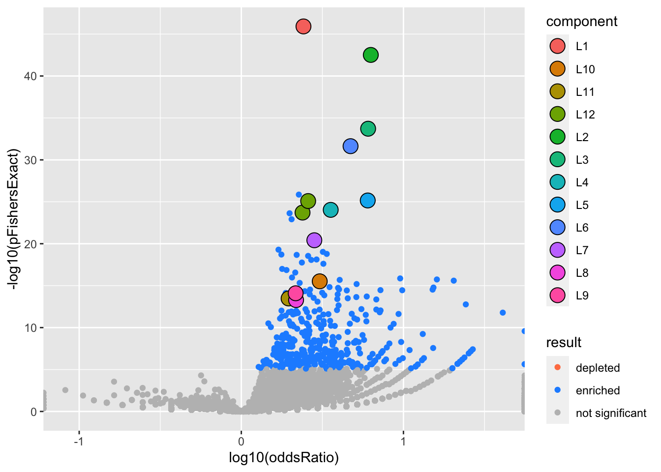
If we account for the predictions made by (logitic) SuSiE, we can see that a lot (but not all of) the enrichment signal has been accounted for.
gseasusie::residual_enrichment_histogram(marginal_regression, residual_regression)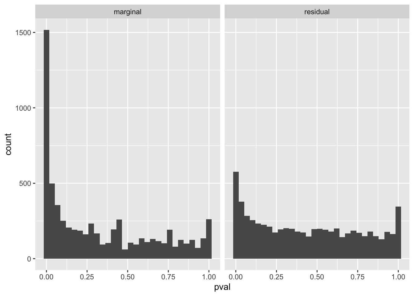
Interactive tables
We can produce an interactive table to explore the enrichment results:
gseasusie::interactive_table(logistic.fit, ora)
sessionInfo()R version 4.1.2 (2021-11-01)
Platform: x86_64-apple-darwin17.0 (64-bit)
Running under: macOS Big Sur 10.16
Matrix products: default
BLAS: /Library/Frameworks/R.framework/Versions/4.1/Resources/lib/libRblas.0.dylib
LAPACK: /Library/Frameworks/R.framework/Versions/4.1/Resources/lib/libRlapack.dylib
locale:
[1] en_US.UTF-8/en_US.UTF-8/en_US.UTF-8/C/en_US.UTF-8/en_US.UTF-8
attached base packages:
[1] stats4 stats graphics grDevices utils datasets methods
[8] base
other attached packages:
[1] DESeq2_1.34.0 SummarizedExperiment_1.24.0
[3] Biobase_2.54.0 MatrixGenerics_1.6.0
[5] matrixStats_0.62.0 GenomicRanges_1.46.1
[7] GenomeInfoDb_1.30.1 IRanges_2.28.0
[9] S4Vectors_0.32.4 BiocGenerics_0.40.0
[11] Matrix_1.4-1 forcats_0.5.1
[13] stringr_1.4.0 dplyr_1.0.9
[15] purrr_0.3.4 readr_2.1.2
[17] tidyr_1.2.0 tibble_3.1.8
[19] ggplot2_3.3.6 tidyverse_1.3.1
[21] gseasusie_0.0.0.9000
loaded via a namespace (and not attached):
[1] colorspace_2.0-3 ellipsis_0.3.2 rprojroot_2.0.3
[4] XVector_0.34.0 fs_1.5.2 rstudioapi_0.13
[7] farver_2.1.1 bit64_4.0.5 mvtnorm_1.1-3
[10] AnnotationDbi_1.56.2 fansi_1.0.3 lubridate_1.8.0
[13] xml2_1.3.3 splines_4.1.2 cachem_1.0.6
[16] geneplotter_1.72.0 knitr_1.39 jsonlite_1.8.0
[19] workflowr_1.7.0 broom_0.8.0 annotate_1.72.0
[22] dbplyr_2.2.0 png_0.1-7 data.tree_1.0.0
[25] compiler_4.1.2 httr_1.4.3 basilisk_1.6.0
[28] tictoc_1.0.1 backports_1.4.1 assertthat_0.2.1
[31] fastmap_1.1.0 cli_3.3.0 later_1.3.0
[34] htmltools_0.5.2 tools_4.1.2 gtable_0.3.0
[37] glue_1.6.2 GenomeInfoDbData_1.2.7 Rcpp_1.0.9
[40] mr.ash.alpha_0.1-42 cellranger_1.1.0 jquerylib_0.1.4
[43] vctrs_0.4.1 Biostrings_2.62.0 crosstalk_1.2.0
[46] xfun_0.31 rvest_1.0.2 irlba_2.3.5
[49] lifecycle_1.0.1 XML_3.99-0.9 org.Hs.eg.db_3.14.0
[52] basilisk.utils_1.6.0 zlibbioc_1.40.0 scales_1.2.0
[55] spatstat.utils_2.3-1 hms_1.1.1 promises_1.2.0.1
[58] parallel_4.1.2 susieR_0.11.92 emulator_1.2-21
[61] RColorBrewer_1.1-3 yaml_2.3.5 reticulate_1.25
[64] memoise_2.0.1 sass_0.4.1 reshape_0.8.9
[67] stringi_1.7.6 RSQLite_2.2.14 highr_0.9
[70] genefilter_1.76.0 filelock_1.0.2 VEB.Boost_0.0.0.9037
[73] BiocParallel_1.28.3 rlang_1.0.4 pkgconfig_2.0.3
[76] bitops_1.0-7 evaluate_0.15 lattice_0.20-45
[79] htmlwidgets_1.5.4 labeling_0.4.2 bit_4.0.4
[82] tidyselect_1.1.2 here_1.0.1 plyr_1.8.7
[85] magrittr_2.0.3 R6_2.5.1 generics_0.1.3
[88] DelayedArray_0.20.0 DBI_1.1.2 pillar_1.8.0
[91] haven_2.5.0 whisker_0.4 withr_2.5.0
[94] mixsqp_0.3-43 survival_3.3-1 KEGGREST_1.34.0
[97] RCurl_1.98-1.7 reactable_0.3.0 dir.expiry_1.2.0
[100] modelr_0.1.8 crayon_1.5.1 utf8_1.2.2
[103] tzdb_0.3.0 rmarkdown_2.14 locfit_1.5-9.5
[106] grid_4.1.2 readxl_1.4.0 reactR_0.4.4
[109] blob_1.2.3 git2r_0.30.1 reprex_2.0.1
[112] digest_0.6.29 xtable_1.8-4 httpuv_1.6.5
[115] munsell_0.5.0 bslib_0.3.1